Algorithms & Complexity
Cheatsheet Content
### Algorithm Basics An **algorithm** is a finite set of well-defined, unambiguous instructions to solve a problem or perform a computation. It must terminate after a finite number of steps and produce a result. #### Estimating & Specifying Execution Times The execution time of an algorithm depends on various factors: - **Input size:** Larger inputs generally take more time. - **Hardware:** Processor speed, memory access. - **Software:** Compiler, operating system. - **Algorithm efficiency:** How well the algorithm uses resources. To provide a machine-independent measure, we use **asymptotic analysis** to estimate the number of basic operations an algorithm performs as a function of its input size, $n$. This gives us a growth rate for the algorithm's runtime. ### Efficiency of Algorithms Algorithm efficiency refers to the amount of resources (time and space) an algorithm consumes to solve a problem. - **Time efficiency:** How fast an algorithm runs, typically measured by the number of basic operations. - **Space efficiency:** How much memory an algorithm uses. #### Methods for Improving Efficiency 1. **Removing redundant computation outside loops:** Move computations that produce the same result in every iteration out of the loop. ```c // Inefficient for (int i = 0; i ### Asymptotic Notations Asymptotic notations describe the limiting behavior of a function as its argument tends towards a particular value or infinity. They are crucial for analyzing algorithm efficiency in a machine-independent way. #### Big-O Notation (O) - Upper Bound - **Definition:** $f(n) = O(g(n))$ if there exist positive constants $c$ and $n_0$ such that $0 \le f(n) \le c \cdot g(n)$ for all $n \ge n_0$. - **Purpose:** Describes the **worst-case** or upper bound of an algorithm's runtime. It tells us that an algorithm will take *at most* a certain amount of time. - **Example:** If an algorithm takes $3n^2 + 2n + 5$ operations, we say it's $O(n^2)$ because for large $n$, $3n^2$ dominates. $$f(n) = 3n^2 + 2n + 5$$ We can choose $c=4$ and $n_0=5$. For $n \ge 5$, $3n^2 + 2n + 5 \le 4n^2$. #### Omega Notation ($\Omega$) - Lower Bound - **Definition:** $f(n) = \Omega(g(n))$ if there exist positive constants $c$ and $n_0$ such that $0 \le c \cdot g(n) \le f(n)$ for all $n \ge n_0$. - **Purpose:** Describes the **best-case** or lower bound of an algorithm's runtime. It tells us that an algorithm will take *at least* a certain amount of time. - **Example:** An algorithm that always takes at least $n \log n$ operations is $\Omega(n \log n)$. $$f(n) = n^2 + 100n$$ We can choose $c=1$ and $n_0=1$. For $n \ge 1$, $n^2 \le n^2 + 100n$. So $f(n) = \Omega(n^2)$. #### Theta Notation ($\Theta$) - Tight Bound - **Definition:** $f(n) = \Theta(g(n))$ if there exist positive constants $c_1, c_2$ and $n_0$ such that $0 \le c_1 \cdot g(n) \le f(n) \le c_2 \cdot g(n)$ for all $n \ge n_0$. - **Purpose:** Describes the **average-case** or tight bound of an algorithm's runtime. It means the algorithm's runtime grows at the same rate as $g(n)$. - **Example:** If an algorithm consistently takes $2n+7$ operations, it's $\Theta(n)$. $$f(n) = 5n + 3$$ We can choose $c_1=5, c_2=6$ and $n_0=3$. For $n \ge 3$, $5n \le 5n+3 \le 6n$. So $f(n) = \Theta(n)$. #### Importance of Asymptotic Notations They allow us to: - **Compare algorithms:** Determine which algorithm is more efficient for large inputs, independent of specific hardware. - **Analyze scalability:** Understand how an algorithm's performance changes as the input size grows. - **Focus on dominant terms:** Ignore lower-order terms and constant factors, which become insignificant for large inputs. ### Loops A **loop** is a control flow statement that allows code to be executed repeatedly based on a boolean condition. #### Aspects in Constructing a Loop 1. **Initialization:** Setting up initial values for loop control variables before the loop begins. *Example:* `int i = 0;` 2. **Condition:** The boolean expression that is evaluated before each iteration. If true, the loop continues; if false, it terminates. *Example:* `i ### Algorithm Strategies Different approaches or paradigms used to design algorithms: 1. **Brute Force:** Tries all possible solutions to a problem to find the optimal one. Often simple to implement but can be inefficient for large inputs. *Example:* Checking every possible permutation to solve the Traveling Salesperson Problem. 2. **Divide and Conquer:** Breaks down a problem into smaller subproblems of the same type, solves them recursively, and then combines their solutions to solve the original problem. *Example:* Merge Sort, Quick Sort, Binary Search. 3. **Dynamic Programming:** Solves problems by breaking them into overlapping subproblems and storing the results of subproblems to avoid redundant computations. *Example:* Fibonacci sequence, knapsack problem. 4. **Greedy Algorithms:** Makes locally optimal choices at each step with the hope of finding a global optimum. Not always guaranteed to find the optimal solution. *Example:* Dijkstra's algorithm, Kruskal's algorithm. 5. **Backtracking:** Explores all potential solutions incrementally, abandoning a path as soon as it determines that it cannot possibly lead to a valid full solution. *Example:* N-Queens problem, Sudoku solver. 6. **Branch and Bound:** Similar to backtracking but for optimization problems. It systematically explores solutions while maintaining bounds on the optimal solution found so far to prune branches that cannot lead to a better solution. *Example:* Solving the Traveling Salesperson Problem, Integer Linear Programming. ### Recursive Algorithms A **recursive algorithm** is an algorithm that calls itself, either directly or indirectly, to solve a problem. It solves a problem by reducing it to smaller instances of the same problem. #### Key Components 1. **Base Case:** A condition that stops the recursion. Without it, the algorithm would run indefinitely (infinite recursion). 2. **Recursive Step:** The part where the function calls itself with a modified (usually smaller) input, moving towards the base case. #### Example: Factorial The factorial of a non-negative integer $n$, denoted $n!$, is the product of all positive integers less than or equal to $n$. $0! = 1$. $$ n! = n \times (n-1)! $$ ```python def factorial_recursive(n): if n == 0: # Base case return 1 else: # Recursive step return n * factorial_recursive(n - 1) # Example usage # factorial_recursive(5) will call: # 5 * factorial_recursive(4) # 5 * (4 * factorial_recursive(3)) # 5 * (4 * (3 * factorial_recursive(2))) # 5 * (4 * (3 * (2 * factorial_recursive(1)))) # 5 * (4 * (3 * (2 * (1 * factorial_recursive(0))))) # 5 * (4 * (3 * (2 * (1 * 1)))) = 120 ``` #### Difference from Iterative Functions | Feature | Recursive Function | Iterative Function | | :--------------- | :----------------------------------------------- | :----------------------------------------------- | | **Structure** | Calls itself; typically uses a base case and recursive step. | Uses loops (for, while) to repeat code. | | **Memory** | Uses a call stack for function calls. Can lead to Stack Overflow for deep recursion. | Uses less memory, typically only for loop variables. | | **Code Length** | Often more concise and elegant for certain problems (e.g., tree traversals). | Can be more verbose for complex problems. | | **Performance** | Can be slower due to function call overhead. | Generally faster due to less overhead. | | **Control Flow** | Managed by system call stack. | Explicitly managed by loops and conditions. | #### Conversion of Iterative to Recursive (and vice-versa) Any iterative function can be converted to a recursive one, and vice-versa. **Example: Iterative Factorial to Recursive** (Recursive example shown above) **Example: Recursive Factorial to Iterative** ```python def factorial_iterative(n): result = 1 for i in range(1, n + 1): result *= i return result # Example usage # factorial_iterative(5) # i=1, result=1 # i=2, result=2 # i=3, result=6 # i=4, result=24 # i=5, result=120 ``` ### UNIT-II: Advanced Algorithm Concepts ### Divide and Conquer **Divide and Conquer (D&C)** is an algorithmic paradigm that solves a problem by recursively breaking it down into two or more subproblems of the same or related type, until these become simple enough to be solved directly. The solutions to the subproblems are then combined to give a solution to the original problem. #### Steps: 1. **Divide:** Break the problem into subproblems that are smaller instances of the same type of problem. 2. **Conquer:** Solve the subproblems recursively. If the subproblems are small enough, solve them directly (base case). 3. **Combine:** Combine the solutions of the subproblems to get the solution for the original problem. #### Example: Merge Sort 1. **Divide:** Split the unsorted list into two halves. 2. **Conquer:** Recursively sort each sublist. 3. **Combine:** Merge the two sorted sublists back into one sorted list. #### Advantages of D&C - **Solving difficult problems:** Can solve problems that are otherwise hard to tackle. - **Efficiency:** Often leads to efficient algorithms (e.g., $O(n \log n)$). - **Parallelism:** Subproblems can often be solved independently, making them suitable for parallel processing. - **Memory Access:** Can improve cache performance due to working on smaller chunks of data. #### Disadvantages of D&C - **Recursion overhead:** Can be slower due to function call overhead. - **Stack overflow:** Deep recursion can lead to stack overflow errors. - **Not always applicable:** Some problems cannot be easily divided into independent subproblems. - **Overlapping subproblems:** If subproblems overlap, it might be less efficient than dynamic programming. #### Characteristics for which D&C is unsuitable D&C is unsuitable when: - **Overlapping Subproblems:** The "divide" step creates many identical subproblems. In such cases, Dynamic Programming is usually more efficient (e.g., calculating Fibonacci numbers recursively is inefficient due to redundant calculations). - **Trivial Base Cases:** The cost of dividing and combining is higher than simply solving the base case directly, even if it's not "small" (e.g., adding two numbers). - **Not decomposable:** The problem cannot be easily broken down into smaller, independent subproblems of the same type. ### Matrix Multiplication The product of two matrices $A$ (of dimensions $m \times p$) and $B$ (of dimensions $p \times n$) is a matrix $C$ (of dimensions $m \times n$). The element $C_{ij}$ is calculated as the dot product of the $i$-th row of $A$ and the $j$-th column of $B$: $$ C_{ij} = \sum_{k=1}^{p} A_{ik} B_{kj} $$ #### Standard Algorithm Time Complexity For two $n \times n$ matrices, the standard algorithm performs $n^3$ multiplications and $n^3 - n^2$ additions. The time complexity is $O(n^3)$. #### Strassen's Matrix Multiplication Strassen's algorithm is a divide and conquer algorithm for matrix multiplication. It significantly reduces the number of scalar multiplications required compared to the standard algorithm. For two $n \times n$ matrices (where $n$ is a power of 2 for simplicity), Strassen's algorithm divides each matrix into four $n/2 \times n/2$ sub-matrices. Instead of 8 recursive multiplications of $n/2 \times n/2$ matrices (as in naive D&C), Strassen's uses 7 special multiplications ($M_1$ to $M_7$) and several additions/subtractions of sub-matrices. **Steps (Simplified):** 1. Divide $A$ and $B$ into $n/2 \times n/2$ sub-matrices: $$ A = \begin{pmatrix} A_{11} & A_{12} \\ A_{21} & A_{22} \end{pmatrix}, \quad B = \begin{pmatrix} B_{11} & B_{12} \\ B_{21} & B_{22} \end{pmatrix} $$ 2. Compute 10 intermediate sub-matrices ($S_1$ to $S_{10}$) using additions/subtractions. 3. Compute 7 products ($P_1$ to $P_7$) of $n/2 \times n/2$ sub-matrices recursively. 4. Compute the four sub-matrices of the result $C$ using additions/subtractions of $P_i$ matrices. $$ C = \begin{pmatrix} C_{11} & C_{12} \\ C_{21} & C_{22} \end{pmatrix} $$ **Strassen's Algorithm Time Complexity:** The recurrence relation for Strassen's algorithm is $T(n) = 7T(n/2) + O(n^2)$. Using the Master Theorem, the time complexity is $O(n^{\log_2 7})$, which is approximately $O(n^{2.807})$. This is better than $O(n^3)$ for large $n$. ### Merge Sort Algorithm Merge Sort is a stable, comparison-based sorting algorithm that follows the Divide and Conquer paradigm. #### How it works: 1. **Divide:** The unsorted list is divided into $n$ sublists, each containing one element (a list of one element is considered sorted). 2. **Conquer (Recursively Sort):** Pair up adjacent sublists and merge them to form new sorted sublists. Repeat until only one sorted list remains. 3. **Combine (Merge):** The merging process compares elements from two sorted sublists and places them into a new sorted list in the correct order. #### Example Walkthrough: `[38, 27, 43, 3, 9, 82, 10]` 1. **Divide:** `[38, 27, 43, 3]` | `[9, 82, 10]` `[38, 27]` | `[43, 3]` || `[9, 82]` | `[10]` `[38]` | `[27]` || `[43]` | `[3]` || `[9]` | `[82]` || `[10]` 2. **Conquer & Combine (Merge):** `[27, 38]` | `[3, 43]` || `[9, 82]` | `[10]` `[3, 27, 38, 43]` || `[9, 10, 82]` `[3, 9, 10, 27, 38, 43, 82]` (Final Sorted List) #### Time Complexity Analysis: - **Divide:** $O(1)$ (just finding the midpoint). - **Conquer:** $2T(n/2)$ (two recursive calls for halves). - **Combine (Merge):** $O(n)$ (linear scan to merge two sorted lists of total size $n$). The recurrence relation is $T(n) = 2T(n/2) + O(n)$. Using the Master Theorem, the time complexity is $O(n \log n)$ in all cases (worst, average, best). Space Complexity: $O(n)$ due to the temporary array used in merging. ### Binary Search Algorithm Binary Search is an efficient algorithm for finding an item from a **sorted list** of items. It works by repeatedly dividing the search interval in half. #### How it works (Divide and Conquer): 1. **Divide:** Compare the target value with the middle element of the sorted array. 2. **Conquer:** * If the target matches the middle element, the search is successful. * If the target is less than the middle element, discard the right half and recursively search in the left half. * If the target is greater than the middle element, discard the left half and recursively search in the right half. 3. **Base Case:** If the interval becomes empty, the item is not found. #### Example: Search for `23` in `[3, 6, 12, 23, 30, 45, 50]` 1. `low = 0, high = 6, mid = 3`. `arr[3] = 23`. Target found! #### Example: Search for `15` in `[3, 6, 12, 23, 30, 45, 50]` 1. `low = 0, high = 6, mid = 3`. `arr[3] = 23`. `15 6`, so search right. 3. `low = 2, high = 2, mid = 2`. `arr[2] = 12`. `15 > 12`, so search right. 4. `low = 3, high = 2`. `low > high`, interval empty. Target not found. #### Time Complexity Analysis: - In each step, the search space is halved. - The number of steps required is $\log_2 n$. - The recurrence relation is $T(n) = T(n/2) + O(1)$. - Using the Master Theorem, the time complexity is $O(\log n)$. Space Complexity: $O(1)$ for iterative version, $O(\log n)$ for recursive version due to call stack. ### Closest Pair Algorithm The closest pair problem is to find the two points (from a set of $n$ points in a 2D plane) that are closest to each other. A naive approach would be to calculate the distance between every pair of points, resulting in $O(n^2)$ complexity. #### Divide and Conquer Approach (Optimal: $O(n \log n)$) 1. **Pre-processing:** Sort all points by their x-coordinates ($P_x$) and y-coordinates ($P_y$). This takes $O(n \log n)$. 2. **Divide:** Divide the set of $n$ points into two equal halves, $P_L$ and $P_R$, by a vertical line $L$ passing through the median x-coordinate. 3. **Conquer:** Recursively find the closest pair in $P_L$ (let its distance be $\delta_L$) and in $P_R$ (let its distance be $\delta_R$). Let $\delta = \min(\delta_L, \delta_R)$. 4. **Combine:** The critical step. The closest pair could be one with points from both $P_L$ and $P_R$. * Consider a "strip" region around the dividing line $L$. This strip contains all points whose x-coordinate is within $\delta$ distance from $L$. Let these points be $P_{strip}$. * Sort $P_{strip}$ by y-coordinate. * For each point $p$ in $P_{strip}$, check only the next 7 (a constant number) points after it in the y-sorted list. This is a crucial optimization; it can be proven that only points within this limited range need to be checked. * Update $\delta$ if a closer pair is found in $P_{strip}$. #### Time Complexity Analysis: - The initial sorting takes $O(n \log n)$. - The recurrence relation for the recursive part is $T(n) = 2T(n/2) + O(n)$, where $O(n)$ comes from merging the y-sorted lists and scanning the strip. - Using the Master Theorem, the recursive part also yields $O(n \log n)$. - Total time complexity: $O(n \log n)$. ### Quick Sort Algorithm Quick Sort is an efficient, in-place, comparison-based sorting algorithm that follows the Divide and Conquer paradigm. It is often faster in practice than other $O(n \log n)$ algorithms like Merge Sort, but its worst-case performance is $O(n^2)$. #### How it works: 1. **Divide (Partition):** Choose an element from the array, called the **pivot**. Rearrange the array such that all elements less than the pivot come before it, and all elements greater than the pivot come after it. Elements equal to the pivot can go on either side. After partitioning, the pivot is in its final sorted position. 2. **Conquer:** Recursively apply Quick Sort to the sub-array of elements with smaller values and separately to the sub-array of elements with greater values. 3. **Base Case:** When a sub-array has zero or one element, it is already sorted. #### Example Walkthrough: `[10, 80, 30, 90, 40, 50, 70]` (Pivot: last element) 1. **Initial:** `[10, 80, 30, 90, 40, 50, 70]` (Pivot = 70) 2. **Partition:** * Elements `[10, 30, 40, 50]` are smaller than 70. * Elements `[80, 90]` are larger than 70. * Result: `[10, 30, 40, 50, 70, 90, 80]` (70 is in its final place) 3. **Conquer (Recursive Calls):** * Quick Sort `[10, 30, 40, 50]` * Quick Sort `[90, 80]` #### Time Complexity Analysis: - **Worst Case:** $O(n^2)$. Occurs when the pivot selection consistently results in highly unbalanced partitions (e.g., already sorted array and pivot is always the smallest/largest element). * Recurrence: $T(n) = T(0) + T(n-1) + O(n) = T(n-1) + O(n)$, which solves to $O(n^2)$. - **Best Case:** $O(n \log n)$. Occurs when the pivot selection consistently divides the array into two roughly equal halves. * Recurrence: $T(n) = 2T(n/2) + O(n)$, which solves to $O(n \log n)$. - **Average Case:** $O(n \log n)$. Due to random pivot selection, the probability of hitting the worst-case scenario repeatedly is very low. Space Complexity: $O(\log n)$ on average (due to recursive call stack), $O(n)$ in worst case.