Load Frequency Control
Cheatsheet Content
### Overview This cheatsheet covers key concepts in Load Frequency Control (LFC) for power systems, including: - Importance of LFC - Schematic diagram of Automatic Generation Control (AGC) - Detailed models of LFC components (Governor, Turbine, Generator) - Complete block diagram of an isolated power system - Steady-state and dynamic analysis - Control Area Concept - Two-Area Load Frequency Control Key components of LFC: - Speed governor system - Turbine - Generator ### Importance of Load Frequency Control - **Continuous Demand Changes:** Active and reactive power demand constantly changes. - **Regulation Requirement:** Steam/water input to generators must be continuously regulated to match active power demand. - **Frequency Stability:** Failure to regulate leads to speed and frequency variations (max $\pm 0.5 \text{Hz}$). - **Parallel Operation:** Maintaining constant network frequency ensures satisfactory parallel operation of power stations. - **Voltage Regulation:** Excitation voltage of generators must be regulated to match reactive power demand, preventing voltages from exceeding limits. **Role of Automatic Load Frequency Control (ALFC):** - Maintain desired megawatt output matching changing load. - Control frequency in larger interconnections. - Keep net interchange power between pool members at predetermined value. - ALFC handles normal (small and slow) load/frequency changes; more drastic emergency control is needed for large imbalances. ### Schematic Diagram of AGC **Description:** This diagram illustrates the integrated control of load frequency and excitation voltage in a turbo-generator. - **Frequency Control Loop:** Senses frequency, compares it with a reference ($f_{ref}$), and adjusts the steam valve controller to regulate steam input to the turbine, thereby controlling the generator's mechanical power output and frequency. - **Excitation Control Loop:** Senses voltage ($V$), compares it with a reference ($V_{ref}$), and adjusts the excitation controller to regulate the generator's field current, thereby controlling reactive power output and voltage. ### Speed Governor System **Components:** - **Fly ball speed governor:** Senses speed (frequency) changes. Fly balls move outwards as speed increases (point B moves downwards), and inwards as speed decreases (point B moves upwards). - **Hydraulic amplifier:** Converts low-power pilot valve movement into high-power main piston movement to open/close the steam valve against high-pressure steam. - **Linkage mechanism (ABC & CDE):** Provides movement to the control valve proportional to speed change and feedback from steam valve movement. - **Speed changer:** Provides steady-state power output setting. Downward movement opens the pilot valve, admitting more steam; upward movement has the reverse effect. ### Model of Speed Governor System The movement of point C is influenced by two factors: 1. **Frequency Increase:** Causes fly balls to move outwards, point B downwards, and consequently point C downwards (proportional to frequency change). 2. **Commanded Power Output Increase:** Causes point A downwards, and consequently point C upwards (proportional to commanded power change). The net movement of C is given by: $$\Delta y_C = -K_1 \Delta P_C + K_2 \Delta f \quad (1)$$ The movement of D, which opens the pilot valve, is contributed by $\Delta y_C$ and $\Delta y_E$: $$\Delta y_D = K_3 \Delta y_C + K_4 \Delta y_E \quad (2)$$ Positive movement of D causes a negative movement of E. The movement of E is obtained by dividing the oil volume by the piston's cross-sectional area: $$\Delta y_E = K_5 \int_0^t -\Delta y_D dt \quad (3)$$ Taking Laplace Transform, we get: $$\Delta Y_C(s) = -K_1 \Delta P_C(s) + K_2 \Delta F(s) \quad (4)$$ $$\Delta Y_D(s) = K_3 \Delta Y_C(s) + K_4 \Delta Y_E(s) \quad (5)$$ $$\Delta Y_E(s) = -K_5 \frac{1}{s} \Delta Y_D(s) \quad (6)$$ Eliminating $\Delta Y_C(s)$ and $\Delta Y_D(s)$: $$\Delta Y_E(s) = \left[ \Delta P_C(s) - \frac{1}{R} \Delta F(s) \right] \times \frac{K_{sg}}{1+T_{sg}s} \quad (7)$$ Where: - $R = K_1/K_2$: Speed regulation of the governor - $K_{sg} = K_1K_3/K_4$: Gain of speed governor - $T_{sg} = 1/(K_4K_5)$: Time constant of speed governor ### Model of Turbine Turbine dynamic response depends on: - Entrained steam between inlet steam valve and first stage. - Storage action in the reheater, causing low-pressure stage output to lag. For simplicity, the turbine can be modeled with a single equivalent time constant: $$\Delta P_T(s) = \frac{K_t}{1+T_t s} \Delta Y_E(s) \quad (8)$$ - $K_t$: Turbine gain - $T_t$: Turbine time constant (typically $0.2 \text{ to } 2.5 \text{ sec}$) ### Model of Generator The increment in power input to the generator-load system ($\Delta P_G - \Delta P_D$) is accounted for in two ways: 1. **Rate of increase of stored kinetic energy in the generator rotor:** $$W_{ke} = W_{ke}^0 \left( \frac{f^0 + \Delta f}{f^0} \right)^2 \approx HP_r \left( 1 + \frac{2\Delta f}{f^0} \right) \quad (9)$$ (Note: $W_{ke}^0 = H \times P_r$) $$\frac{d}{dt} (\Delta W_{ke}) = \frac{2HP_r}{f^0} \frac{d}{dt} (\Delta f) \quad (10)$$ 2. **Rate of change of motor loads (considered constant for small frequency changes):** $$\left( \frac{\partial P_D}{\partial f} \right) \Delta f = B \Delta f \quad (11)$$ **Power balance equation:** $$\Delta P_G - \Delta P_D = \frac{2HP_r}{f^0} \frac{d}{dt} (\Delta f) + B \Delta f \quad (12)$$ Dividing throughout by $P_r$: $$\Delta P_G(pu) - \Delta P_D(pu) = \frac{2H}{f^0} \frac{d}{dt} (\Delta f) + B(pu) \Delta f \quad (13)$$ Taking Laplace Transform and rearranging: $$\Delta F(s) = \frac{\Delta P_G(s) - \Delta P_D(s)}{B + \frac{2H}{f^0}s} \quad (14)$$ This can be written as: $$\Delta F(s) = [\Delta P_G(s) - \Delta P_D(s)] \times \frac{K_{ps}}{1+T_{ps}s} \quad (15)$$ Where: - $K_{ps} = 1/B$: Power system gain - $T_{ps} = 2H/(Bf^0)$: Power system time constant ### Complete Block Diagram of an Isolated Power System This diagram combines the models of the governor, turbine, and generator to represent the load frequency control of an isolated power system. - $\Delta P_C(s)$: Change in commanded power - $\Delta F(s)$: Change in frequency - $\Delta P_D(s)$: Change in load demand ### Steady-State Analysis of an Isolated Power System Two incremental inputs for LFC: 1. Change in speed changer setting ($\Delta P_C$) 2. Change in load demand ($\Delta P_D$) **Case (a): Speed changer fixed ($\Delta P_C = 0$) - Free Governor Operation** For a sudden change in load demand $\Delta P_D$ ($\Delta P_D(s) = \Delta P_D/s$): $$\Delta F(s)|_{\Delta P_C(s)=0} = \frac{\Delta P_D(s)}{s} \times \frac{K_{ps}}{1 + T_{ps}s + \frac{K_{sg}K_tK_{ps}}{R} \frac{1}{1+T_{sg}s)(1+T_t s)}} \quad (16)$$ The steady-state frequency change is: $$\Delta f|_{\text{steady state}, \Delta P_C=0} = -\frac{1}{B + 1/R} \Delta P_D \quad (18)$$ This equation shows the linear relationship between frequency and load for free governor operation. **Case (b): Load demand fixed ($\Delta P_D = 0$)** For a change in speed changer setting $\Delta P_C$ ($\Delta P_C(s) = \Delta P_C/s$): $$\Delta F(s)|_{\Delta P_D(s)=0} = \frac{\Delta P_C(s)}{s} \times \frac{K_{sg}K_tK_{ps}/(1+T_{sg}s)(1+T_t s)}{1 + T_{ps}s + \frac{K_{sg}K_tK_{ps}}{R} \frac{1}{1+T_{sg}s)(1+T_t s)}} \quad (19)$$ If $K_{sg}K_t \approx 1$, the steady-state frequency change is: $$\Delta f = - \left( \frac{1}{B+1/R} \right) \Delta P_C \quad (21)$$ ### Dynamic Response of an Isolated Power System The characteristic equation can be approximated to first order by examining time constants: $T_{sg} This shows the frequency drop and its recovery to a new steady-state value after a load change. ### Control Area Concept - **Definition:** A large power system is divided into subareas where generators are tightly coupled, forming a **coherent group**. - **Frequency Uniformity:** In a control area, frequency is assumed to be uniform under static and dynamic conditions. - **Strict Specifications:** System frequency specifications are stringent, and significant frequency changes are not tolerated. - **Goal:** Steady-state frequency change is expected to be zero. **Role of Automatic Adjustment:** - Speed changer setting is automatically adjusted to monitor frequency change. - Change in frequency is fed through an integrator to achieve zero steady-state error. - The error in frequency in LFC for a given control area is known as **Area Control Error (ACE)**. This figure illustrates the dynamic response of the LFC system with and without integral control, showing how integral control helps eliminate steady-state error. ### Two-Area Load Frequency Control **Control Objectives:** - Regulate frequency of each area. - Regulate the tie-line power as per inter-area power contract. **Incremental Power Accounts For:** - Rate of increase of stored kinetic energy. - Increase in area load due to frequency increase. - Tie-line transport of power in or out of an area. **Power Transported Out of Area 1:** $$P_{tie,1} = \frac{|V_1||V_2|}{X_{12}} \sin(\delta_1^0 - \delta_2^0) \quad (24)$$ Where $\delta_1^0, \delta_2^0$ are power angles of equivalent machines. **Incremental Tie-Line Power for Changes in $\delta_1, \delta_2$:** $$\Delta P_{tie,1}(pu) = T_{12}(\Delta \delta_1 - \Delta \delta_2) \quad (25)$$ Where $T_{12} = \frac{|V_1||V_2|}{P_r X_{12}} \cos(\delta_1^0 - \delta_2^0)$ is the synchronizing coefficient. This can be rewritten as: $$\Delta P_{tie,1} = 2\pi T_{12} \left( \int \Delta f_1 dt - \int \Delta f_2 dt \right) \quad (26)$$ **Laplace Transform of Incremental Tie-Line Power:** $$\Delta P_{tie,1}(s) = \frac{2\pi T_{12}}{s} (\Delta F_1(s) - \Delta F_2(s)) \quad (30)$$ Similarly for Area 2: $$\Delta P_{tie,2}(s) = -\frac{2\pi T_{12}}{s} (\Delta F_1(s) - \Delta F_2(s)) \quad (31)$$ **Incremental Power Balance Equation for Area 1:** $$\Delta P_{G1} - \Delta P_{D1} = \frac{2H_1}{f^0} \frac{d}{dt} (\Delta f_1) + B_1 \Delta f_1 + \Delta P_{tie,1} \quad (28)$$ Taking Laplace Transform: $$\Delta F_1(s) = [\Delta P_{G1}(s) - \Delta P_{D1}(s) - \Delta P_{tie,1}(s)] \times \frac{K_{ps1}}{1+T_{ps1}s} \quad (29)$$ Where $K_{ps1} = 1/B_1$ and $T_{ps1} = 2H_1/(B_1f^0)$. **Area Control Error (ACE):** With an additional integral control loop to make steady-state tie-line power zero, ACE is redefined. For Control Area 1: $$ACE_1 = \Delta P_{tie,1} + b_1 \Delta f_1 \quad (32)$$ $$ACE_1(s) = \Delta P_{tie,1}(s) + b_1 \Delta F_1(s) \quad (33)$$ For Control Area 2: $$ACE_2 = \Delta P_{tie,2} + b_2 \Delta f_2 \quad (34)$$ $$ACE_2(s) = \Delta P_{tie,2}(s) + b_2 \Delta F_2(s) \quad (35)$$ Where $b_1$ and $b_2$ are area frequency bias constants. This composite block diagram shows the feedback loops with integral control for two-area LFC, incorporating ACE to achieve zero steady-state error.