Quantum Mechanics-I Pass Guide

Cheatsheet Content

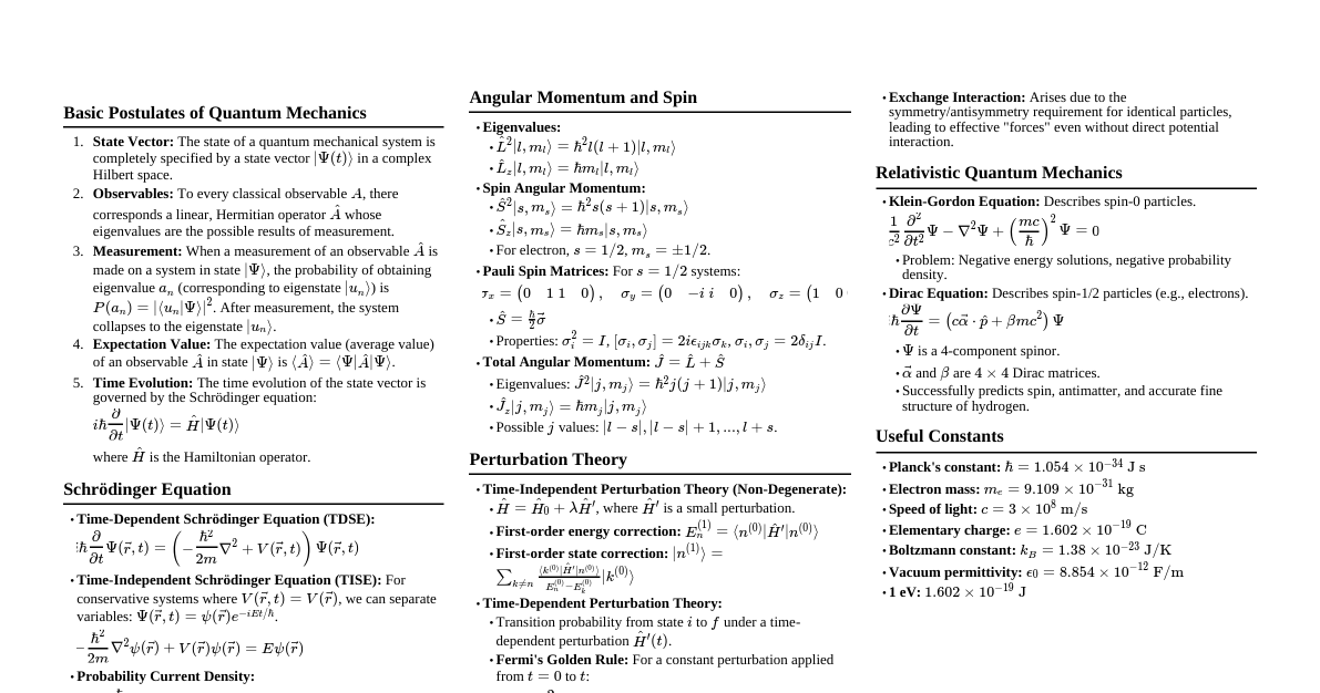
### Introduction to Quantum Mechanics-I: Pass Guide (MPH-004) This guide is designed to help M.Sc. (Physics) students efficiently prepare for and pass the MPH-004 Quantum Mechanics-I examination. The content is curated based on analysis of previous year question papers and assignments from 2023, 2024, 2025, and 2026, focusing on frequently asked, high-weightage topics. The goal is to maximize your score with minimum preparation time. #### How to Use This Guide 1. **Prioritize:** Focus on "VERY IMPORTANT" and "IMPORTANT" topics first. "LOW PRIORITY" topics can be skipped if time is short. 2. **Understand Concepts:** Read the simple theory explanations to grasp the core ideas. 3. **Memorize Formulas:** Keep the key equations and formula lists handy. Understand the symbols and applications. 4. **Practice Derivations:** Follow the step-by-step derivations. Practice writing them out without referring to the guide. 5. **Solve Problems:** Work through the solved problems. Understand the method and try similar problems. 6. **Attempt Expected Questions:** Use the provided questions for self-assessment and practice writing exam-ready answers. 7. **Last Minute Revision:** Utilize the quick revision sheets and formula summaries for a final brush-up before the exam. ### Smart Study Plan This plan prioritizes topics based on their frequency and weightage in past examinations. #### Phase 1: Core Concepts (VERY IMPORTANT) - High Priority * **Wave-Particle Duality & Uncertainty Principle:** Fundamental to QM. Always asked. * **Schrödinger Equation (Time-Independent & Dependent):** Derivations and applications are crucial. * **One-Dimensional Potentials:** Particle in a Box (Infinite & Finite), Harmonic Oscillator. These are recurring problem types. * **Hydrogen Atom:** Eigenfunctions, eigenvalues, expectation values. * **Angular Momentum:** Operators, commutation relations, eigenvalues, eigenvectors. * **Operators & Observables:** Hermitian operators, expectation values, commutation relations. #### Phase 2: Advanced Concepts (IMPORTANT) - Medium Priority * **Matrix Representation of Operators:** Calculation of matrix elements, diagonalization. * **Perturbation Theory (Time-Independent):** Understanding the concept and first-order corrections. * **Spin:** Pauli spin matrices, spin angular momentum. * **Scattering Theory (Basic Concepts):** Cross-section, phase shifts (if time permits). #### Phase 3: Supplementary Topics (LOW PRIORITY) - Low Priority * Specialized potentials or advanced mathematical techniques not frequently tested. #### Time Management Strategy * **Focus on Derivations:** Many questions involve deriving key equations. Master these. * **Practice Problem Solving:** Numericals from 1D potentials and Hydrogen atom are common. * **Write Down Answers:** Practice structuring your answers for 5 and 10-mark questions. * **Don't Skip Fundamentals:** A strong grasp of Phase 1 topics is essential for passing. * **If Time is Very Limited:** Concentrate solely on "VERY IMPORTANT" topics, especially derivations and conceptual questions. ### Physical Constants (Provided in Exam) It is useful to know these common values: * Planck's constant ($h$) = $6.626 \times 10^{-34}$ Js * Reduced Planck's constant ($\hbar$) = $1.05 \times 10^{-34}$ Js (or $h/2\pi$) * Mass of electron ($m_e$) = $9.11 \times 10^{-31}$ kg * Mass of proton ($m_p$) = $1.67 \times 10^{-27}$ kg * Mass of neutron ($m_n$) = $1.675 \times 10^{-27}$ kg * Elementary charge ($e$) = $1.6 \times 10^{-19}$ C * Boltzmann constant ($k_B$) = $1.38 \times 10^{-23}$ JK$^{-1}$ ### Wave-Particle Duality and De Broglie Wavelength (VERY IMPORTANT) #### Theory Explanation Wave-particle duality is a fundamental concept in quantum mechanics stating that every particle or quantum entity may be partly described in terms of waves and partly in terms of particles. The de Broglie hypothesis, proposed by Louis de Broglie, states that all matter exhibits wave-like properties, and relates the wavelength of a particle to its momentum. #### Important Definitions * **De Broglie Wavelength ($\lambda$):** The wavelength associated with a particle, given by $\lambda = h/p$, where $h$ is Planck's constant and $p$ is the momentum of the particle. * **Wave-Particle Duality:** The concept that particles can exhibit wave-like properties and waves can exhibit particle-like properties. #### Key Equations and Formula List 1. **De Broglie Wavelength:** $$\lambda = \frac{h}{p} = \frac{h}{mv}$$ * $h$: Planck's constant * $p$: momentum of the particle * $m$: mass of the particle * $v$: velocity of the particle 2. **Kinetic Energy (for non-relativistic particles):** $$KE = \frac{1}{2}mv^2 = \frac{p^2}{2m}$$ * Used to find momentum $p = \sqrt{2mKE}$. 3. **For thermal particles (e.g., nitrogen molecule at room temperature):** $$KE = \frac{3}{2}k_BT$$ * $k_B$: Boltzmann constant * $T$: Absolute temperature in Kelvin 4. **For electrons accelerated through a potential V:** $$KE = eV$$ * $e$: Elementary charge * $V$: Accelerating potential #### Problem-Solving Method (Frequently Asked) **Example:** Calculate the de Broglie wavelength of a nitrogen molecule at room temperature ($T = 300 K$), given that the mass of a nitrogen molecule is $4.65 \times 10^{-26}$ kg. **Formula Used:** $\lambda = \frac{h}{\sqrt{2mKE}}$ and $KE = \frac{3}{2}k_BT$ **Step-by-step Solution:** 1. **Calculate Kinetic Energy:** $KE = \frac{3}{2}k_BT = \frac{3}{2} \times (1.38 \times 10^{-23} \text{ JK}^{-1}) \times (300 \text{ K})$ $KE = 6.21 \times 10^{-21}$ J 2. **Calculate Momentum:** $p = \sqrt{2mKE} = \sqrt{2 \times (4.65 \times 10^{-26} \text{ kg}) \times (6.21 \times 10^{-21} \text{ J})}$ $p = \sqrt{5.775 \times 10^{-46}}$ $p \approx 2.40 \times 10^{-23}$ kg m/s 3. **Calculate de Broglie Wavelength:** $\lambda = \frac{h}{p} = \frac{6.626 \times 10^{-34} \text{ Js}}{2.40 \times 10^{-23} \text{ kg m/s}}$ $\lambda \approx 2.76 \times 10^{-11}$ m = 0.0276 nm **Explanation:** * Step 1 uses the equipartition theorem for thermal energy. * Step 2 relates kinetic energy to momentum. * Step 3 applies the de Broglie hypothesis. #### Expected Exam Questions * **5-mark:** Calculate the de Broglie wavelength for (a) an electron accelerated by 100V, (b) a proton moving at $10^6$ m/s, or (c) a thermal neutron at 300K. (High Probability) * **5-mark:** Explain wave-particle duality and its significance in quantum mechanics. * **2-mark:** What is the de Broglie hypothesis? ### Heisenberg's Uncertainty Principle (VERY IMPORTANT) #### Theory Explanation Heisenberg's Uncertainty Principle states that it is impossible to simultaneously determine with perfect accuracy certain pairs of conjugate variables, such as position ($x$) and momentum ($p_x$), or energy ($E$) and time ($t$). The more precisely one variable is known, the less precisely the other can be known. #### Important Definitions * **Conjugate Variables:** Pairs of physical properties that cannot be simultaneously known to high precision. * **Uncertainty ($\Delta x$, $\Delta p_x$, $\Delta E$, $\Delta t$):** The standard deviation or spread in the measurement of a physical quantity. #### Key Equations and Formula List 1. **Position-Momentum Uncertainty:** $$\Delta x \Delta p_x \ge \frac{\hbar}{2}$$ * $\Delta x$: Uncertainty in position * $\Delta p_x$: Uncertainty in momentum * $\hbar$: Reduced Planck's constant 2. **Energy-Time Uncertainty:** $$\Delta E \Delta t \ge \frac{\hbar}{2}$$ * $\Delta E$: Uncertainty in energy * $\Delta t$: Uncertainty in time (e.g., lifetime of a state) #### Problem-Solving Method (Frequently Asked) **Example:** Estimate the uncertainty in the energy of a photon localized within a distance of 0.1 nm. **Formula Used:** $\Delta x \Delta p_x \ge \frac{\hbar}{2}$ and $E = pc$ (for photon) $\implies \Delta E = c \Delta p_x$ **Step-by-step Solution:** 1. **Identify given uncertainty:** $\Delta x = 0.1 \text{ nm} = 0.1 \times 10^{-9} \text{ m} = 10^{-10} \text{ m}$. 2. **Use uncertainty principle for momentum:** $\Delta p_x \ge \frac{\hbar}{2\Delta x}$ $\Delta p_x \ge \frac{1.05 \times 10^{-34} \text{ Js}}{2 \times 10^{-10} \text{ m}}$ $\Delta p_x \ge 5.25 \times 10^{-25}$ kg m/s 3. **Relate momentum uncertainty to energy uncertainty (for photon):** For a photon, $E = pc$, so $\Delta E = c \Delta p_x$. $\Delta E \ge (3 \times 10^8 \text{ m/s}) \times (5.25 \times 10^{-25} \text{ kg m/s})$ $\Delta E \ge 1.575 \times 10^{-16}$ J **Explanation:** * Step 1 identifies the given position uncertainty. * Step 2 applies the position-momentum uncertainty principle to find the minimum momentum uncertainty. * Step 3 converts momentum uncertainty to energy uncertainty using the photon energy-momentum relation. **Example 2: Zero-point energy using Uncertainty Principle (Frequently Asked)** Estimate the zero-point energy of a particle of mass $m$ confined to move in a one-dimensional region between two infinitely high potential barriers separated by a distance $L_0$. **Formula Used:** $\Delta x \Delta p_x \ge \frac{\hbar}{2}$ and $E = \frac{p^2}{2m}$ **Step-by-step Solution:** 1. **Estimate $\Delta x$:** The particle is confined within $L_0$. So, the uncertainty in position is approximately $\Delta x \approx L_0$. 2. **Estimate $\Delta p_x$:** From the uncertainty principle, $\Delta p_x \ge \frac{\hbar}{2L_0}$. Since the particle is confined, its average momentum is zero, but it must have some momentum fluctuation. Thus, the minimum momentum $p \approx \Delta p_x$. 3. **Estimate Zero-Point Energy:** $E_{min} = \frac{p^2}{2m} \approx \frac{(\Delta p_x)^2}{2m} \ge \frac{(\hbar/(2L_0))^2}{2m}$ $E_{min} \ge \frac{\hbar^2}{8mL_0^2}$ **Explanation:** * For a confined particle, its position uncertainty is roughly the confinement length. * The minimum momentum is associated with the minimum uncertainty. * This minimum energy is the "zero-point energy," implying that even at absolute zero, a confined quantum particle has non-zero energy. #### Expected Exam Questions * **5-mark:** State and explain Heisenberg's Uncertainty Principle. * **5-mark:** Using the uncertainty principle, estimate the zero-point energy of a one-dimensional harmonic oscillator or a particle in a box. (High Probability) * **5-mark:** Estimate the minimum kinetic energy of an electron confined to a region of size 0.1 nm (atomic size). * **2-mark:** What are conjugate variables? Give an example. ### Schrödinger Equation (VERY IMPORTANT) #### Theory Explanation The Schrödinger equation is a mathematical equation that describes how the quantum state of a physical system changes over time. It is a central equation in quantum mechanics, analogous to Newton's laws of motion in classical mechanics. It exists in two main forms: time-dependent and time-independent. #### Important Definitions * **Wave Function ($\Psi$ or $\psi$):** A mathematical function that describes the quantum state of a particle. Its square magnitude ($|\Psi|^2$) gives the probability density of finding the particle at a given position and time. * **Hamiltonian Operator ($\hat{H}$):** The operator corresponding to the total energy of the system. * **Stationary State:** A quantum state in which the probability density $|\Psi|^2$ is constant over time. These are solutions to the time-independent Schrödinger equation. #### Key Equations and Formula List 1. **Time-Dependent Schrödinger Equation (TDSE):** $$i\hbar \frac{\partial \Psi(\vec{r}, t)}{\partial t} = \hat{H} \Psi(\vec{r}, t)$$ Where $\hat{H} = -\frac{\hbar^2}{2m}\nabla^2 + V(\vec{r}, t)$ * $\Psi(\vec{r}, t)$: Time-dependent wave function * $\hat{H}$: Hamiltonian operator * $V(\vec{r}, t)$: Potential energy function 2. **Time-Independent Schrödinger Equation (TISE):** $$\hat{H} \psi(\vec{r}) = E \psi(\vec{r})$$ Where $\hat{H} = -\frac{\hbar^2}{2m}\nabla^2 + V(\vec{r})$ * $\psi(\vec{r})$: Time-independent wave function (eigenfunction) * $E$: Energy eigenvalue * $V(\vec{r})$: Potential energy function (independent of time) 3. **General Solution for TDSE (for time-independent potential):** $$\Psi(\vec{r}, t) = \psi(\vec{r}) e^{-iEt/\hbar}$$ #### Important Derivations (High Probability) **Derivation of Time-Dependent Schrödinger Equation:** 1. **Start with classical energy:** $E = KE + PE = \frac{p^2}{2m} + V$ 2. **Introduce quantum operators:** * Energy operator: $\hat{E} = i\hbar \frac{\partial}{\partial t}$ * Momentum operator: $\hat{p} = -i\hbar \nabla$ * Position operator: $\hat{r} = \vec{r}$ 3. **Substitute operators into energy equation and apply to wave function $\Psi$:** $$i\hbar \frac{\partial \Psi}{\partial t} = \frac{(-i\hbar \nabla)^2}{2m} \Psi + V \Psi$$ $$i\hbar \frac{\partial \Psi}{\partial t} = -\frac{\hbar^2}{2m}\nabla^2 \Psi + V \Psi$$ $$i\hbar \frac{\partial \Psi}{\partial t} = \left(-\frac{\hbar^2}{2m}\nabla^2 + V\right) \Psi$$ $$i\hbar \frac{\partial \Psi}{\partial t} = \hat{H} \Psi$$ **Assumptions:** Non-relativistic particle, potential energy $V$ can be time-dependent. **Final Result:** The Time-Dependent Schrödinger Equation. **Derivation of Time-Independent Schrödinger Equation from TDSE:** 1. **Assume separable solution:** $\Psi(\vec{r}, t) = \psi(\vec{r}) T(t)$ for a time-independent potential $V(\vec{r})$. 2. **Substitute into TDSE:** $$i\hbar \psi(\vec{r}) \frac{dT(t)}{dt} = \left(-\frac{\hbar^2}{2m}\nabla^2 + V(\vec{r})\right) \psi(\vec{r}) T(t)$$ 3. **Divide by $\psi(\vec{r}) T(t)$:** $$\frac{i\hbar}{T(t)} \frac{dT(t)}{dt} = \frac{1}{\psi(\vec{r})} \left(-\frac{\hbar^2}{2m}\nabla^2 + V(\vec{r})\right) \psi(\vec{r})$$ 4. **Equate both sides to a constant (E, energy):** Since the left side depends only on $t$ and the right side only on $\vec{r}$, both must be equal to a constant, which we call $E$. * **Time part:** $i\hbar \frac{dT(t)}{dt} = ET(t) \implies T(t) = e^{-iEt/\hbar}$ * **Spatial part:** $-\frac{\hbar^2}{2m}\nabla^2 \psi(\vec{r}) + V(\vec{r}) \psi(\vec{r}) = E \psi(\vec{r})$ $$\hat{H} \psi(\vec{r}) = E \psi(\vec{r})$$ **Assumptions:** Separable solution, time-independent potential. **Final Result:** The Time-Independent Schrödinger Equation. #### Problem-Solving (Determining Potential from Wavefunction) **Example:** A quantum mechanical particle in one dimension has the wave function: $\psi(x) = Nx^n$ for $x > 0$ and $n > 1$. Use the Schrödinger equation to determine the corresponding potential $V(x)$. **Formula Used:** Time-Independent Schrödinger Equation: $-\frac{\hbar^2}{2m}\frac{d^2\psi}{dx^2} + V(x)\psi(x) = E\psi(x)$ **Step-by-step Solution:** 1. **Find the first derivative of $\psi(x)$:** $\frac{d\psi}{dx} = Nnx^{n-1}$ 2. **Find the second derivative of $\psi(x)$:** $\frac{d^2\psi}{dx^2} = Nn(n-1)x^{n-2}$ 3. **Substitute into TISE:** $-\frac{\hbar^2}{2m} [Nn(n-1)x^{n-2}] + V(x)[Nx^n] = E[Nx^n]$ 4. **Divide by $Nx^n$ (assuming $N \ne 0$ and $x \ne 0$):** $-\frac{\hbar^2}{2m} n(n-1)x^{-2} + V(x) = E$ 5. **Solve for $V(x)$:** $V(x) = E + \frac{\hbar^2 n(n-1)}{2m x^2}$ **Explanation:** * We use the TISE because the wavefunction is time-independent. * By calculating the derivatives and substituting them into the equation, we can isolate $V(x)$. * The resulting potential is a combination of a constant energy $E$ and an inverse square potential, which often arises in central force problems. #### Expected Exam Questions * **10-mark:** Derive the time-dependent Schrödinger equation. Explain the physical significance of the wave function. (Very Important) * **10-mark:** Derive the time-independent Schrödinger equation from the time-dependent one. Explain stationary states. (Very Important) * **5-mark:** Given a wave function, determine the potential $V(x)$ or the energy $E$. (High Probability, similar to example) * **5-mark:** What is the Hamiltonian operator? Write it for a free particle and a particle in a potential $V(x)$. * **2-mark:** What is a stationary state? ### Normalization and Expectation Values (VERY IMPORTANT) #### Theory Explanation * **Normalization:** For a physically realistic wave function, the total probability of finding the particle somewhere in space must be 1. This condition is called normalization. * **Expectation Value:** The average value of a physical quantity (observable) if measured many times on an ensemble of identical systems. In quantum mechanics, it is calculated using the wave function and the corresponding operator. #### Important Definitions * **Probability Density:** $|\Psi(\vec{r},t)|^2$ or $|\psi(\vec{r})|^2$, representing the probability per unit volume of finding the particle at $\vec{r}$ at time $t$. * **Normalization Condition:** $\int |\Psi(\vec{r},t)|^2 d\tau = 1$ (integrated over all space). * **Expectation Value of an Operator $\hat{A}$:** $\langle \hat{A} \rangle = \int \Psi^* \hat{A} \Psi d\tau$. #### Key Equations and Formula List 1. **Normalization Condition (1D):** $$\int_{-\infty}^{\infty} |\psi(x)|^2 dx = 1$$ 2. **Expectation Value of Position (1D):** $$\langle x \rangle = \int_{-\infty}^{\infty} \psi^*(x) x \psi(x) dx$$ 3. **Expectation Value of Momentum (1D):** $$\langle p_x \rangle = \int_{-\infty}^{\infty} \psi^*(x) \left(-i\hbar \frac{\partial}{\partial x}\right) \psi(x) dx$$ 4. **Expectation Value of Energy (1D):** $$\langle E \rangle = \int_{-\infty}^{\infty} \psi^*(x) \left(-\frac{\hbar^2}{2m}\frac{\partial^2}{\partial x^2} + V(x)\right) \psi(x) dx$$ #### Problem-Solving Method (Frequently Asked) **Example 1: Normalization (Frequently Asked)** Normalize the wave function: $\psi(x,0) = N \left(\sin\left(\frac{\pi x}{L}\right) + \sin\left(\frac{2\pi x}{L}\right)\right)$, for $0 \le x ### Operators and Observables (VERY IMPORTANT) #### Theory Explanation In quantum mechanics, every measurable physical quantity (observable) is associated with a linear, Hermitian operator. The eigenvalues of these operators correspond to the possible results of measurement, and the eigenfunctions are the states in which the observable has a definite value. #### Important Definitions * **Observable:** A physical quantity that can be measured (e.g., position, momentum, energy). * **Operator:** A mathematical instruction that transforms one function into another. * **Hermitian Operator:** An operator $\hat{A}$ for which $\int \psi_1^* (\hat{A}\psi_2) d\tau = \int (\hat{A}\psi_1)^* \psi_2 d\tau$. Hermitian operators have real eigenvalues and their eigenfunctions corresponding to distinct eigenvalues are orthogonal. * **Commutator:** The commutator of two operators $\hat{A}$ and $\hat{B}$ is $[\hat{A}, \hat{B}] = \hat{A}\hat{B} - \hat{B}\hat{A}$. If the commutator is zero, the operators commute, and the corresponding observables can be measured simultaneously with arbitrary precision. #### Key Equations and Formula List 1. **Position Operator:** $\hat{x} = x$ 2. **Momentum Operator:** $\hat{p}_x = -i\hbar \frac{\partial}{\partial x}$ 3. **Kinetic Energy Operator:** $\hat{T} = -\frac{\hbar^2}{2m}\frac{\partial^2}{\partial x^2}$ 4. **Potential Energy Operator:** $\hat{V} = V(x)$ 5. **Hamiltonian Operator:** $\hat{H} = \hat{T} + \hat{V}$ 6. **Commutation Relation for Position and Momentum:** $[\hat{x}, \hat{p}_x] = i\hbar$ 7. **Commutator of Angular Momentum Operators:** * $[\hat{L}_x, \hat{L}_y] = i\hbar \hat{L}_z$ * $[\hat{L}_y, \hat{L}_z] = i\hbar \hat{L}_x$ * $[\hat{L}_z, \hat{L}_x] = i\hbar \hat{L}_y$ #### Important Derivations (High Probability) **Show that $[\hat{x}, \hat{p}_x] = i\hbar$:** 1. **Apply commutator to an arbitrary test function $f(x)$:** $[\hat{x}, \hat{p}_x]f(x) = (\hat{x}\hat{p}_x - \hat{p}_x\hat{x})f(x)$ 2. **Substitute operators:** $= x(-i\hbar \frac{\partial}{\partial x})f(x) - (-i\hbar \frac{\partial}{\partial x})(x f(x))$ $= -i\hbar x \frac{\partial f}{\partial x} - (-i\hbar) \left( f(x) + x \frac{\partial f}{\partial x} \right)$ $= -i\hbar x \frac{\partial f}{\partial x} + i\hbar f(x) + i\hbar x \frac{\partial f}{\partial x}$ $= i\hbar f(x)$ 3. **Conclusion:** Since $[\hat{x}, \hat{p}_x]f(x) = i\hbar f(x)$ for any $f(x)$, we have $[\hat{x}, \hat{p}_x] = i\hbar$. **Assumptions:** Standard definitions of position and momentum operators. **Final Result:** The fundamental commutation relation between position and momentum. **Show that if $\hat{O}$ is Hermitian and $\hat{U}$ is unitary, then $\hat{U}\hat{O}\hat{U}^{-1}$ is Hermitian:** 1. **Definition of Hermitian operator:** $\hat{A}$ is Hermitian if $\hat{A}^\dagger = \hat{A}$. 2. **Definition of Unitary operator:** $\hat{U}$ is unitary if $\hat{U}^\dagger = \hat{U}^{-1}$. 3. **Consider the adjoint of $\hat{U}\hat{O}\hat{U}^{-1}$:** $(\hat{U}\hat{O}\hat{U}^{-1})^\dagger = (\hat{U}^{-1})^\dagger \hat{O}^\dagger \hat{U}^\dagger$ 4. **Apply unitary property:** $(\hat{U}^{-1})^\dagger = (\hat{U}^\dagger)^\dagger = \hat{U}$. So, $(\hat{U}\hat{O}\hat{U}^{-1})^\dagger = \hat{U} \hat{O}^\dagger \hat{U}^\dagger$ 5. **Apply Hermitian property of $\hat{O}$ and unitary property of $\hat{U}$:** $\hat{O}^\dagger = \hat{O}$ and $\hat{U}^\dagger = \hat{U}^{-1}$. $(\hat{U}\hat{O}\hat{U}^{-1})^\dagger = \hat{U} \hat{O} \hat{U}^{-1}$ 6. **Conclusion:** Since the adjoint of $\hat{U}\hat{O}\hat{U}^{-1}$ is equal to itself, it is Hermitian. **Final Result:** A transformed Hermitian operator by a unitary transformation remains Hermitian. #### Problem-Solving (Commutators) **Example:** Show that $[\hat{L}_x\hat{L}_y, \hat{L}_z] = i\hbar (\hat{L}_x^2 - \hat{L}_y^2)$. (Frequently Asked) **Formula Used:** Commutator properties: $[AB, C] = A[B,C] + [A,C]B$ Angular momentum commutators: $[\hat{L}_x, \hat{L}_y] = i\hbar \hat{L}_z$, $[\hat{L}_y, \hat{L}_z] = i\hbar \hat{L}_x$, $[\hat{L}_z, \hat{L}_x] = i\hbar \hat{L}_y$ **Step-by-step Solution:** 1. **Apply commutator property:** $[\hat{L}_x\hat{L}_y, \hat{L}_z] = \hat{L}_x[\hat{L}_y, \hat{L}_z] + [\hat{L}_x, \hat{L}_z]\hat{L}_y$ 2. **Substitute known angular momentum commutators:** * $[\hat{L}_y, \hat{L}_z] = i\hbar \hat{L}_x$ * $[\hat{L}_x, \hat{L}_z] = -[\hat{L}_z, \hat{L}_x] = -i\hbar \hat{L}_y$ 3. **Substitute back into the expression:** $= \hat{L}_x (i\hbar \hat{L}_x) + (-i\hbar \hat{L}_y) \hat{L}_y$ $= i\hbar \hat{L}_x^2 - i\hbar \hat{L}_y^2$ $= i\hbar (\hat{L}_x^2 - \hat{L}_y^2)$ **Explanation:** * This problem tests the understanding of commutator properties and the fundamental commutation relations of angular momentum operators. * Careful application of these rules leads to the desired result. #### Expected Exam Questions * **5-mark:** Explain what a Hermitian operator is. Show that its eigenvalues are real. (Very Important) * **5-mark:** Show that the position and momentum operators do not commute, i.e., $[\hat{x}, \hat{p}_x] = i\hbar$. (Very Important) * **5-mark:** Show that if $\hat{A}$ is Hermitian, then $\hat{A}^2$ is also Hermitian. * **5-mark:** Calculate the commutator of given operators, e.g., $[\hat{L}_x\hat{L}_y, \hat{L}_z]$. (High Probability) * **5-mark:** Define Hermitian and anti-Hermitian operators. For an operator $\hat{A}$, show that $(\hat{A} + \hat{A}^\dagger)$ is Hermitian and $(\hat{A} - \hat{A}^\dagger)$ is anti-Hermitian. * **2-mark:** What is an observable in quantum mechanics? ### One-Dimensional Potentials: Particle in a Box (VERY IMPORTANT) #### Theory Explanation The particle in a box model describes a particle confined to a small region of space surrounded by impenetrable barriers. It is one of the simplest quantum mechanical problems that demonstrates the quantization of energy levels and the existence of zero-point energy. #### Important Definitions * **Infinite Potential Well:** A region where the potential energy is zero inside the box and infinite outside, meaning the particle cannot escape. * **Eigenfunctions:** The allowed wave functions of the particle in the box. * **Eigenvalues:** The allowed discrete energy levels of the particle in the box. #### Key Equations and Formula List 1. **Potential for Infinite Square Well (length L):** $$V(x) = \begin{cases} 0 & 0 \le x \le L \\ \infty & \text{otherwise} \end{cases}$$ 2. **Energy Eigenvalues:** $$E_n = \frac{n^2\pi^2\hbar^2}{2mL^2}, \quad n = 1, 2, 3, \ldots$$ 3. **Normalized Wavefunctions:** $$\psi_n(x) = \sqrt{\frac{2}{L}} \sin\left(\frac{n\pi x}{L}\right), \quad n = 1, 2, 3, \ldots$$ #### Important Derivations (High Probability) **Derivation of Energy Eigenvalues and Eigenfunctions for 1D Infinite Potential Well:** 1. **Set up TISE:** For $0 \le x \le L$, $V(x)=0$, so the TISE is: $$-\frac{\hbar^2}{2m}\frac{d^2\psi}{dx^2} = E\psi$$ $$\frac{d^2\psi}{dx^2} + k^2\psi = 0, \quad \text{where } k^2 = \frac{2mE}{\hbar^2}$$ 2. **General Solution:** $\psi(x) = A\sin(kx) + B\cos(kx)$ 3. **Apply Boundary Conditions:** * $\psi(0) = 0 \implies A\sin(0) + B\cos(0) = 0 \implies B=0$. So, $\psi(x) = A\sin(kx)$. * $\psi(L) = 0 \implies A\sin(kL) = 0$. Since $A \ne 0$ (for non-trivial solution), $\sin(kL)=0$. This implies $kL = n\pi$, where $n = 1, 2, 3, \ldots$ (n=0 gives trivial solution). So, $k = \frac{n\pi}{L}$. 4. **Determine Energy Eigenvalues:** Substitute $k$ back into $k^2 = \frac{2mE}{\hbar^2}$: $$\left(\frac{n\pi}{L}\right)^2 = \frac{2mE_n}{\hbar^2} \implies E_n = \frac{n^2\pi^2\hbar^2}{2mL^2}$$ 5. **Normalize Wavefunctions:** Use $\int_0^L |\psi_n(x)|^2 dx = 1$: $\int_0^L A^2 \sin^2\left(\frac{n\pi x}{L}\right) dx = 1$ $A^2 \frac{L}{2} = 1 \implies A = \sqrt{\frac{2}{L}}$ So, $\psi_n(x) = \sqrt{\frac{2}{L}} \sin\left(\frac{n\pi x}{L}\right)$. **Assumptions:** Particle confined to a 1D box with infinite walls. **Final Result:** Quantized energy levels and sinusoidal wavefunctions. #### Problem-Solving (Odd Parity State) **Example:** Calculate the expectation values $\langle x \rangle$ and $\langle x^2 \rangle$ for the following odd parity state of a symmetric infinite potential well: $\psi(x) = \frac{1}{\sqrt{a}} \sin\left(\frac{n\pi x}{2a}\right)$ for $n=2,4,6,...$ (This implies a box from $-a$ to $a$). **Formula Used:** $\langle x \rangle = \int_{-a}^{a} \psi^*(x) x \psi(x) dx$ $\langle x^2 \rangle = \int_{-a}^{a} \psi^*(x) x^2 \psi(x) dx$ **Step-by-step Solution:** 1. **For $\langle x \rangle$:** $\langle x \rangle = \int_{-a}^{a} \frac{1}{a} \sin^2\left(\frac{n\pi x}{2a}\right) x dx$ The integrand $f(x) = x \sin^2\left(\frac{n\pi x}{2a}\right)$ is an odd function because $x$ is odd and $\sin^2(\cdot)$ is even. The integral of an odd function over a symmetric interval $[-a, a]$ is zero. Therefore, $\langle x \rangle = 0$. 2. **For $\langle x^2 \rangle$:** $\langle x^2 \rangle = \int_{-a}^{a} \frac{1}{a} x^2 \sin^2\left(\frac{n\pi x}{2a}\right) dx$ The integrand $g(x) = x^2 \sin^2\left(\frac{n\pi x}{2a}\right)$ is an even function. This integral is more complex and usually involves known standard integrals or integration by parts. For a particle in a box of length $L$ (from $0$ to $L$), $\langle x^2 \rangle = \frac{L^2}{3} - \frac{L^2}{2n^2\pi^2}$. For a box from $-a$ to $a$, the length is $L=2a$. So, $\langle x^2 \rangle = \frac{(2a)^2}{3} - \frac{(2a)^2}{2n^2\pi^2} = \frac{4a^2}{3} - \frac{2a^2}{n^2\pi^2}$. **Explanation:** * The symmetry of the potential and the parity of the integrand are crucial for $\langle x \rangle$. For a symmetric potential, $\langle x \rangle = 0$ for any energy eigenstate. * $\langle x^2 \rangle$ measures the spread of the particle's position. #### Expected Exam Questions * **10-mark:** Derive the energy eigenvalues and normalized wave functions for a particle in a one-dimensional infinite potential well. (Very Important) * **5-mark:** Calculate the expectation values $\langle x \rangle$ and $\langle p_x \rangle$ for the ground state of a particle in a 1D infinite potential well. * **5-mark:** Discuss the implications of the zero-point energy for a particle in a box. * **2-mark:** What are the boundary conditions for a particle in an infinite potential well? ### One-Dimensional Potentials: Harmonic Oscillator (VERY IMPORTANT) #### Theory Explanation The quantum harmonic oscillator is a model system in quantum mechanics that describes the behavior of a particle subjected to a quadratic potential. It is one of the most important models as it approximates various physical systems, such as molecular vibrations and lattice vibrations in solids. #### Important Definitions * **Harmonic Potential:** $V(x) = \frac{1}{2}m\omega^2 x^2$. * **Annihilation Operator ($\hat{a}$):** Lowers the energy of a state by $\hbar\omega$. * **Creation Operator ($\hat{a}^\dagger$):** Raises the energy of a state by $\hbar\omega$. * **Number Operator ($\hat{N}$):** $\hat{N} = \hat{a}^\dagger\hat{a}$, its eigenvalues are the quantum numbers $n$. #### Key Equations and Formula List 1. **Hamiltonian:** $$\hat{H} = -\frac{\hbar^2}{2m}\frac{d^2}{dx^2} + \frac{1}{2}m\omega^2 x^2$$ 2. **Energy Eigenvalues:** $$E_n = \left(n + \frac{1}{2}\right)\hbar\omega, \quad n = 0, 1, 2, \ldots$$ 3. **Ground State Wavefunction ($n=0$):** $$\psi_0(x) = \left(\frac{m\omega}{\pi\hbar}\right)^{1/4} e^{-m\omega x^2 / (2\hbar)}$$ 4. **Raising and Lowering Operators:** $$\hat{a} = \sqrt{\frac{m\omega}{2\hbar}} \left(\hat{x} + \frac{i}{m\omega}\hat{p}_x\right)$$ $$\hat{a}^\dagger = \sqrt{\frac{m\omega}{2\hbar}} \left(\hat{x} - \frac{i}{m\omega}\hat{p}_x\right)$$ 5. **Commutation Relation:** $[\hat{a}, \hat{a}^\dagger] = 1$ 6. **Action of Ladder Operators on Energy Eigenstates:** $$\hat{a}|n\rangle = \sqrt{n}|n-1\rangle$$ $$\hat{a}^\dagger|n\rangle = \sqrt{n+1}|n+1\rangle$$ #### Important Derivations (High Probability) **Show that $[\hat{H}, \hat{a}] = -\hbar\omega\hat{a}$ (and similar for $\hat{a}^\dagger$):** 1. **Express $\hat{H}$ in terms of $\hat{a}$ and $\hat{a}^\dagger$:** From the definitions of $\hat{a}$ and $\hat{a}^\dagger$: $\hat{x} = \sqrt{\frac{\hbar}{2m\omega}}(\hat{a} + \hat{a}^\dagger)$ $\hat{p}_x = i\sqrt{\frac{m\omega\hbar}{2}}(\hat{a}^\dagger - \hat{a})$ Substitute these into $\hat{H} = \frac{\hat{p}_x^2}{2m} + \frac{1}{2}m\omega^2 \hat{x}^2$. After algebra and using $[\hat{a}, \hat{a}^\dagger] = 1$, we get: $$\hat{H} = \hbar\omega \left(\hat{a}^\dagger\hat{a} + \frac{1}{2}\right)$$ 2. **Calculate the commutator $[\hat{H}, \hat{a}]$:** $[\hat{H}, \hat{a}] = \left[\hbar\omega \left(\hat{a}^\dagger\hat{a} + \frac{1}{2}\right), \hat{a}\right]$ $= \hbar\omega [\hat{a}^\dagger\hat{a}, \hat{a}]$ $= \hbar\omega (\hat{a}^\dagger[\hat{a}, \hat{a}] + [\hat{a}^\dagger, \hat{a}]\hat{a})$ 3. **Use $[\hat{a}, \hat{a}] = 0$ and $[\hat{a}^\dagger, \hat{a}] = -[\hat{a}, \hat{a}^\dagger] = -1$:** $= \hbar\omega (0 + (-1)\hat{a})$ $= -\hbar\omega \hat{a}$ Similarly, $[\hat{H}, \hat{a}^\dagger] = \hbar\omega \hat{a}^\dagger$. **Assumptions:** Standard definitions of Hamiltonian and ladder operators. **Final Result:** Commutation relations between Hamiltonian and ladder operators, showing they raise/lower energy by $\hbar\omega$. #### Problem-Solving (Expectation Value of Potential Energy) **Example:** Calculate the expectation value of the potential energy for the first excited state of a simple harmonic oscillator. **Formula Used:** $V(x) = \frac{1}{2}m\omega^2 x^2$ $\hat{x} = \sqrt{\frac{\hbar}{2m\omega}}(\hat{a} + \hat{a}^\dagger)$ $\langle V \rangle = \langle n | \frac{1}{2}m\omega^2 \hat{x}^2 | n \rangle$ For the first excited state, $n=1$. **Step-by-step Solution:** 1. **Express $\hat{x}^2$ in terms of ladder operators:** $\hat{x}^2 = \frac{\hbar}{2m\omega}(\hat{a} + \hat{a}^\dagger)^2 = \frac{\hbar}{2m\omega}(\hat{a}^2 + \hat{a}\hat{a}^\dagger + \hat{a}^\dagger\hat{a} + (\hat{a}^\dagger)^2)$ Using $\hat{a}\hat{a}^\dagger = \hat{a}^\dagger\hat{a} + 1$: $\hat{x}^2 = \frac{\hbar}{2m\omega}(\hat{a}^2 + 2\hat{a}^\dagger\hat{a} + 1 + (\hat{a}^\dagger)^2)$ 2. **Substitute into $\langle V \rangle$ for $n=1$ state:** $\langle V \rangle = \langle 1 | \frac{1}{2}m\omega^2 \frac{\hbar}{2m\omega}(\hat{a}^2 + 2\hat{a}^\dagger\hat{a} + 1 + (\hat{a}^\dagger)^2) | 1 \rangle$ $\langle V \rangle = \frac{1}{4}\hbar\omega \langle 1 | \hat{a}^2 + 2\hat{a}^\dagger\hat{a} + 1 + (\hat{a}^\dagger)^2 | 1 \rangle$ 3. **Apply ladder operators:** * $\hat{a}^2|1\rangle = \hat{a}(\sqrt{1}|0\rangle) = \hat{a}|0\rangle = 0$ * $\hat{a}^\dagger\hat{a}|1\rangle = \hat{N}|1\rangle = 1|1\rangle$ * $(\hat{a}^\dagger)^2|1\rangle = \hat{a}^\dagger(\sqrt{2}|2\rangle) = \sqrt{2}\sqrt{3}|3\rangle = \sqrt{6}|3\rangle$ 4. **Evaluate the expectation value (using orthogonality $\langle n|m \rangle = \delta_{nm}$):** $\langle V \rangle = \frac{1}{4}\hbar\omega \left(\langle 1 | 0 \rangle + 2\langle 1 | 1 \rangle + \langle 1 | 1 \rangle + \langle 1 | \sqrt{6}|3\rangle \right)$ $\langle V \rangle = \frac{1}{4}\hbar\omega (0 + 2(1) + 1 + 0)$ $\langle V \rangle = \frac{1}{4}\hbar\omega (3) = \frac{3}{4}\hbar\omega$ Alternatively, for any state $|n\rangle$, $\langle V \rangle = \frac{1}{2} E_n = \frac{1}{2} \left(n + \frac{1}{2}\right)\hbar\omega$. For $n=1$, $\langle V \rangle = \frac{1}{2} \left(1 + \frac{1}{2}\right)\hbar\omega = \frac{1}{2} \left(\frac{3}{2}\right)\hbar\omega = \frac{3}{4}\hbar\omega$. **Explanation:** * This problem demonstrates the power of using ladder operators to simplify calculations involving expectation values for the harmonic oscillator. * The expectation value of potential energy for any energy eigenstate is half of its total energy. #### Expected Exam Questions * **10-mark:** Explain the ladder operator method for the 1D quantum harmonic oscillator. Derive the energy eigenvalues using this method. (Very Important) * **5-mark:** Show that $[\hat{H}, \hat{a}] = -\hbar\omega\hat{a}$ and $[\hat{H}, \hat{a}^\dagger] = \hbar\omega\hat{a}^\dagger$. (High Probability) * **5-mark:** Calculate the expectation value of potential energy ($\langle V \rangle$) or kinetic energy ($\langle T \rangle$) for a given state of the harmonic oscillator. (High Probability) * **5-mark:** Calculate the matrix element $\langle n | \hat{x} | n+1 \rangle$ or $\langle n | \hat{p}_x | n+1 \rangle$. * **2-mark:** What is the zero-point energy of a harmonic oscillator? ### Hydrogen Atom (VERY IMPORTANT) #### Theory Explanation The hydrogen atom is the simplest atomic system, consisting of a proton and an electron. Its quantum mechanical treatment provides a fundamental understanding of atomic structure, quantization of energy, angular momentum, and electron orbitals. #### Important Definitions * **Principal Quantum Number ($n$):** Determines the energy level ($n=1,2,3,...$). * **Orbital Angular Momentum Quantum Number ($l$):** Determines the magnitude of angular momentum ($l=0,1,...,n-1$). * **Magnetic Quantum Number ($m_l$):** Determines the z-component of angular momentum ($m_l=-l, ..., 0, ..., l$). * **Degeneracy:** Multiple distinct quantum states having the same energy. For hydrogen, the energy levels depend only on $n$, so states with different $l$ and $m_l$ but the same $n$ are degenerate. #### Key Equations and Formula List 1. **Energy Eigenvalues:** $$E_n = -\frac{me^4}{8\epsilon_0^2 h^2 n^2} = -\frac{13.6}{n^2} \text{ eV}, \quad n = 1, 2, 3, \ldots$$ * $m$: reduced mass of electron-proton system (approx mass of electron) * $e$: elementary charge * $\epsilon_0$: permittivity of free space * $h$: Planck's constant 2. **Eigenfunctions (separated into radial and angular parts):** $$\psi_{nlm_l}(r, \theta, \phi) = R_{nl}(r) Y_{lm_l}(\theta, \phi)$$ * $R_{nl}(r)$: Radial wave function (depends on $n, l$) * $Y_{lm_l}(\theta, \phi)$: Spherical harmonics (depends on $l, m_l$) 3. **Angular Momentum Squared Operator Eigenvalues:** $$\hat{L}^2 Y_{lm_l}(\theta, \phi) = l(l+1)\hbar^2 Y_{lm_l}(\theta, \phi)$$ 4. **Z-component Angular Momentum Operator Eigenvalues:** $$\hat{L}_z Y_{lm_l}(\theta, \phi) = m_l\hbar Y_{lm_l}(\theta, \phi)$$ 5. **Bohr Radius ($a_0$):** $$a_0 = \frac{4\pi\epsilon_0\hbar^2}{me^2} \approx 0.0529 \text{ nm}$$ #### Problem-Solving (Eigenfunctions, Eigenvalues, Most Probable Value) **Example:** For the hydrogen atom: i) Write down the eigenfunctions for the $300$ and $310$ states. ii) Write the eigenvalues of $\hat{L}^2$ and $\hat{L}_z$ for the states $300$ and $310$. iii) Calculate the most probable value of $r$ for the hydrogen atom in the state $210$. **Formula Used:** * $\psi_{nlm_l}(r, \theta, \phi) = R_{nl}(r) Y_{lm_l}(\theta, \phi)$ * $\hat{L}^2 Y_{lm_l}(\theta, \phi) = l(l+1)\hbar^2 Y_{lm_l}(\theta, \phi)$ * $\hat{L}_z Y_{lm_l}(\theta, \phi) = m_l\hbar Y_{lm_l}(\theta, \phi)$ * Most probable $r$ is found by maximizing $P(r) = r^2 |R_{nl}(r)|^2$. **Step-by-step Solution:** i) **Eigenfunctions:** * **For $300$ state:** $n=3, l=0, m_l=0$. $\psi_{300}(r, \theta, \phi) = R_{30}(r) Y_{00}(\theta, \phi)$ $Y_{00} = \frac{1}{\sqrt{4\pi}}$ $R_{30}(r) = \frac{2}{81\sqrt{3}a_0^{3/2}} (27 - 18\frac{r}{a_0} + 2\frac{r^2}{a_0^2}) e^{-r/(3a_0)}$ (Exact forms of $R_{nl}$ are usually provided or not required for simple questions, focus on the general form and quantum numbers) * **For $310$ state:** $n=3, l=1, m_l=0$. $\psi_{310}(r, \theta, \phi) = R_{31}(r) Y_{10}(\theta, \phi)$ $Y_{10} = \sqrt{\frac{3}{4\pi}} \cos\theta$ $R_{31}(r) = \frac{4}{81\sqrt{6}a_0^{3/2}} (6\frac{r}{a_0} - \frac{r^2}{a_0^2}) e^{-r/(3a_0)}$ ii) **Eigenvalues of $\hat{L}^2$ and $\hat{L}_z$:** * **For $300$ state ($l=0, m_l=0$):** $\hat{L}^2 \psi_{300} = 0(0+1)\hbar^2 \psi_{300} = 0$ $\hat{L}_z \psi_{300} = 0\hbar \psi_{300} = 0$ * **For $310$ state ($l=1, m_l=0$):** $\hat{L}^2 \psi_{310} = 1(1+1)\hbar^2 \psi_{310} = 2\hbar^2 \psi_{310}$ $\hat{L}_z \psi_{310} = 0\hbar \psi_{310} = 0$ iii) **Most probable value of $r$ for $210$ state:** ($n=2, l=1, m_l=0$) The radial wave function is $R_{21}(r) = \frac{1}{\sqrt{3}(2a_0)^{3/2}} \frac{r}{a_0} e^{-r/(2a_0)}$. The radial probability density is $P(r) = r^2 |R_{21}(r)|^2 = C r^4 e^{-r/a_0}$. To find the most probable value, set $\frac{dP(r)}{dr} = 0$: $\frac{d}{dr} (C r^4 e^{-r/a_0}) = C (4r^3 e^{-r/a_0} - \frac{1}{a_0} r^4 e^{-r/a_0}) = 0$ $C r^3 e^{-r/a_0} (4 - \frac{r}{a_0}) = 0$ This gives $r=0$ (minimum) or $r \to \infty$ (minimum), or $4 - \frac{r}{a_0} = 0$. So, $r = 4a_0$. **Explanation:** * Understanding the quantum numbers ($n, l, m_l$) is key to identifying the state. * Eigenvalues of angular momentum operators depend only on $l$ and $m_l$. * The most probable radial distance involves maximizing the radial probability density $P(r) = r^2 |R_{nl}(r)|^2$. #### Expected Exam Questions * **10-mark:** Write down the eigenvalue equations for the operators $\hat{H}$, $\hat{L}^2$, and $\hat{L}_z$ for the hydrogen atom. List the eigenfunctions for $n=3$. What is the number of degenerate eigenfunctions for $n=3$? (Very Important) * **5-mark:** Calculate the expectation value of $r$ or $1/r$ for a given state of the hydrogen atom (e.g., ground state). * **5-mark:** Determine the most probable value of $r$ for a given hydrogen atom state. (High Probability) * **2-mark:** What is the physical significance of the quantum numbers $n, l, m_l$? ### Angular Momentum (VERY IMPORTANT) #### Theory Explanation Angular momentum is a fundamental observable in quantum mechanics. Unlike classical angular momentum, its magnitude and components are quantized. The theory of angular momentum is crucial for understanding atomic and molecular spectra, as well as spin. #### Important Definitions * **Angular Momentum Operators ($\hat{L}_x, \hat{L}_y, \hat{L}_z$):** Operators corresponding to the components of orbital angular momentum. * **Total Angular Momentum Operator ($\hat{L}^2$):** Operator corresponding to the square of the total orbital angular momentum. * **Ladder Operators ($\hat{L}_+, \hat{L}_-$):** $\hat{L}_+ = \hat{L}_x + i\hat{L}_y$ (raising operator) and $\hat{L}_- = \hat{L}_x - i\hat{L}_y$ (lowering operator). * **Eigenstates:** States $|l, m_l\rangle$ that are simultaneous eigenstates of $\hat{L}^2$ and $\hat{L}_z$. #### Key Equations and Formula List 1. **Orbital Angular Momentum Operators (Cartesian):** * $\hat{L}_x = -i\hbar\left(y\frac{\partial}{\partial z} - z\frac{\partial}{\partial y}\right)$ * $\hat{L}_y = -i\hbar\left(z\frac{\partial}{\partial x} - x\frac{\partial}{\partial z}\right)$ * $\hat{L}_z = -i\hbar\left(x\frac{\partial}{\partial y} - y\frac{\partial}{\partial x}\right)$ 2. **Commutation Relations (already covered in Operators section):** * $[\hat{L}_x, \hat{L}_y] = i\hbar \hat{L}_z$ (cyclic permutations apply) * $[\hat{L}^2, \hat{L}_x] = 0$ (and for $\hat{L}_y, \hat{L}_z$) 3. **Eigenvalues:** * $\hat{L}^2 |l, m_l\rangle = l(l+1)\hbar^2 |l, m_l\rangle$ * $\hat{L}_z |l, m_l\rangle = m_l\hbar |l, m_l\rangle$ * where $l = 0, 1, 2, \ldots$ and $m_l = -l, -l+1, \ldots, l$. 4. **Action of Ladder Operators:** * $\hat{L}_+ |l, m_l\rangle = \hbar \sqrt{l(l+1) - m_l(m_l+1)} |l, m_l+1\rangle$ * $\hat{L}_- |l, m_l\rangle = \hbar \sqrt{l(l+1) - m_l(m_l-1)} |l, m_l-1\rangle$ #### Important Derivations (High Probability) **Derive the matrix elements of $\hat{J}_x, \hat{J}_y, \hat{J}_z$ for $j=1/2$ (Spin 1/2 system):** 1. **Define basis states:** For $j=1/2$, the possible $m_j$ values are $+1/2$ and $-1/2$. Let's denote them as $|\uparrow\rangle = |1/2, 1/2\rangle$ and $|\downarrow\rangle = |1/2, -1/2\rangle$. 2. **Matrix elements of $\hat{J}_z$:** $\hat{J}_z |\uparrow\rangle = (1/2)\hbar |\uparrow\rangle$ $\hat{J}_z |\downarrow\rangle = (-1/2)\hbar |\downarrow\rangle$ So, $\hat{J}_z = \frac{\hbar}{2} \begin{pmatrix} 1 & 0 \\ 0 & -1 \end{pmatrix} = \frac{\hbar}{2}\sigma_z$. 3. **Matrix elements of $\hat{J}_+$ and $\hat{J}_-$, then $\hat{J}_x, \hat{J}_y$:** * $\hat{J}_+ |j, m_j\rangle = \hbar \sqrt{j(j+1)-m_j(m_j+1)} |j, m_j+1\rangle$ * $\hat{J}_- |j, m_j\rangle = \hbar \sqrt{j(j+1)-m_j(m_j-1)} |j, m_j-1\rangle$ For $j=1/2$: * $\hat{J}_+ |\downarrow\rangle = \hbar \sqrt{1/2(3/2) - (-1/2)(1/2)} |\uparrow\rangle = \hbar \sqrt{3/4 + 1/4} |\uparrow\rangle = \hbar |\uparrow\rangle$ * $\hat{J}_+ |\uparrow\rangle = 0$ * $\hat{J}_- |\uparrow\rangle = \hbar \sqrt{1/2(3/2) - (1/2)(-1/2)} |\downarrow\rangle = \hbar \sqrt{3/4 + 1/4} |\downarrow\rangle = \hbar |\downarrow\rangle$ * $\hat{J}_- |\downarrow\rangle = 0$ In matrix form: $\hat{J}_+ = \hbar \begin{pmatrix} 0 & 1 \\ 0 & 0 \end{pmatrix}$ $\hat{J}_- = \hbar \begin{pmatrix} 0 & 0 \\ 1 & 0 \end{pmatrix}$ Now, $\hat{J}_x = \frac{1}{2}(\hat{J}_+ + \hat{J}_-)$ and $\hat{J}_y = \frac{1}{2i}(\hat{J}_+ - \hat{J}_-)$. $\hat{J}_x = \frac{\hbar}{2} \begin{pmatrix} 0 & 1 \\ 1 & 0 \end{pmatrix} = \frac{\hbar}{2}\sigma_x$ $\hat{J}_y = \frac{\hbar}{2i} \begin{pmatrix} 0 & 1 \\ -1 & 0 \end{pmatrix} = \frac{\hbar}{2} \begin{pmatrix} 0 & -i \\ i & 0 \end{pmatrix} = \frac{\hbar}{2}\sigma_y$ **Final Result:** The spin matrices (Pauli matrices) for spin 1/2. #### Problem-Solving (Action of Ladder Operators) **Example:** For the angular momentum state $|3,1\rangle$, show that $\hat{J}_+|3,1\rangle = \hbar\sqrt{10}|3,2\rangle$ and $\hat{J}_-|3,1\rangle = 2\hbar\sqrt{3}|3,0\rangle$. **Formula Used:** * $\hat{J}_+ |j, m_j\rangle = \hbar \sqrt{j(j+1) - m_j(m_j+1)} |j, m_j+1\rangle$ * $\hat{J}_- |j, m_j\rangle = \hbar \sqrt{j(j+1) - m_j(m_j-1)} |j, m_j-1\rangle$ **Step-by-step Solution:** 1. **For $\hat{J}_+|3,1\rangle$:** Here $j=3, m_j=1$. $\hat{J}_+|3,1\rangle = \hbar \sqrt{3(3+1) - 1(1+1)} |3,1+1\rangle$ $= \hbar \sqrt{3(4) - 1(2)} |3,2\rangle$ $= \hbar \sqrt{12 - 2} |3,2\rangle = \hbar \sqrt{10} |3,2\rangle$ 2. **For $\hat{J}_-|3,1\rangle$:** Here $j=3, m_j=1$. $\hat{J}_-|3,1\rangle = \hbar \sqrt{3(3+1) - 1(1-1)} |3,1-1\rangle$ $= \hbar \sqrt{3(4) - 1(0)} |3,0\rangle$ $= \hbar \sqrt{12 - 0} |3,0\rangle = \hbar \sqrt{12} |3,0\rangle = 2\hbar\sqrt{3}|3,0\rangle$ **Explanation:** * Direct application of the ladder operator formulas with the given quantum numbers $j$ and $m_j$. * This confirms how ladder operators change the $m_j$ quantum number while keeping $j$ constant. #### Expected Exam Questions * **10-mark:** Write down the angular momentum states $|j, m_j\rangle$. Calculate the matrix elements of $\hat{J}_x, \hat{J}_y, \hat{J}_z$ for $j=1/2$. (Very Important) * **5-mark:** Show the commutation relations for angular momentum operators: $[\hat{L}_x, \hat{L}_y] = i\hbar \hat{L}_z$. * **5-mark:** Explain the action of angular momentum ladder operators $\hat{L}_+$ and $\hat{L}_-$. Apply them to a given angular momentum state. (High Probability) * **5-mark:** Write down the angular momentum states $|j, m_j\rangle$ for $j=2$ and the eigenvalue of $\hat{J}^2$ and $\hat{J}_z$ for each of these states. * **2-mark:** Why do $\hat{L}^2$ and $\hat{L}_z$ commute? ### Matrix Representation of Operators (IMPORTANT) #### Theory Explanation In quantum mechanics, operators and states can be represented as matrices and vectors, respectively, in a chosen basis. This matrix formulation is particularly useful for systems with a finite number of states (e.g., spin systems) or for understanding operator properties. #### Important Definitions * **Basis Vectors:** A set of orthonormal states that span the Hilbert space of the system. * **Matrix Element of Operator $\hat{A}$:** $\langle i | \hat{A} | j \rangle$, where $|i\rangle$ and $|j\rangle$ are basis vectors. * **Spectral Representation:** Expressing an operator in terms of its eigenvalues and eigenvectors, e.g., $\hat{A} = \sum_n a_n |n\rangle \langle n|$ where $a_n$ are eigenvalues and $|n\rangle$ are eigenvectors. #### Key Equations and Formula List 1. **Matrix Element:** $$A_{ij} = \langle i | \hat{A} | j \rangle$$ 2. **Operator in Matrix Form (for a finite basis):** $$\hat{A} = \sum_{i,j} |i\rangle A_{ij} \langle j|$$ 3. **Inner Product of State Vectors (for column vectors):** If $|\psi\rangle = \begin{pmatrix} c_1 \\ c_2 \end{pmatrix}$ and $|\phi\rangle = \begin{pmatrix} d_1 \\ d_2 \end{pmatrix}$, then $\langle \phi | \psi \rangle = (d_1^* \ d_2^*) \begin{pmatrix} c_1 \\ c_2 \end{pmatrix} = d_1^*c_1 + d_2^*c_2$. 4. **Norm of a State Vector:** $\|\psi\| = \sqrt{\langle \psi | \psi \rangle}$ #### Problem-Solving (State Vectors and Matrix Elements) **Example:** Consider the following state vectors: $|\psi\rangle = \begin{pmatrix} 1 \\ -i \end{pmatrix}$ and $|\phi\rangle = \begin{pmatrix} i \\ 1-i \end{pmatrix}$. Calculate (i) the norm of $|\psi\rangle$ and (ii) the inner product $\langle \phi | \psi \rangle$. **Formula Used:** * Norm: $\| \psi \| = \sqrt{\langle \psi | \psi \rangle}$ * Inner product: $\langle \phi | \psi \rangle = \phi^\dagger \psi$ **Step-by-step Solution:** i) **Norm of $|\psi\rangle$:** $\langle \psi | = (1 \ \ i)$ $\langle \psi | \psi \rangle = (1 \ \ i) \begin{pmatrix} 1 \\ -i \end{pmatrix} = (1)(1) + (i)(-i) = 1 - i^2 = 1 - (-1) = 2$ $\|\psi\| = \sqrt{2}$ ii) **Inner product $\langle \phi | \psi \rangle$:** $\langle \phi | = (-i \ \ 1+i)$ $\langle \phi | \psi \rangle = (-i \ \ 1+i) \begin{pmatrix} 1 \\ -i \end{pmatrix} = (-i)(1) + (1+i)(-i)$ $= -i -i + (-i^2) = -2i + 1 = 1 - 2i$ **Explanation:** * The adjoint of a column vector is a row vector with complex conjugate elements. * Matrix multiplication rules are applied for inner products. **Example 2: Matrix Elements from Spectral Representation** A Hermitian operator $\hat{A}$ in a basis $|1\rangle, |2\rangle$ is given by the spectral representation: $\hat{A} = 3|1\rangle\langle1| - |2\rangle\langle2|$. For a normalized state given by $|\chi\rangle = \frac{1}{2}|1\rangle + \frac{\sqrt{3}}{2}|2\rangle$, calculate $\langle \hat{A} \rangle$ and the root mean square deviation in $\hat{A}$. **Formula Used:** * $\langle \hat{A} \rangle = \langle \chi | \hat{A} | \chi \rangle$ * $(\Delta A)^2 = \langle \hat{A}^2 \rangle - \langle \hat{A} \rangle^2$ **Step-by-step Solution:** 1. **Calculate $\langle \hat{A} \rangle$:** $\langle \hat{A} \rangle = \left( \frac{1}{2}\langle 1| + \frac{\sqrt{3}}{2}\langle 2| \right) (3|1\rangle\langle1| - |2\rangle\langle2|) \left( \frac{1}{2}|1\rangle + \frac{\sqrt{3}}{2}|2\rangle \right)$ $= \left( \frac{1}{2}\langle 1| + \frac{\sqrt{3}}{2}\langle 2| \right) \left( \frac{3}{2}|1\rangle - \frac{\sqrt{3}}{2}|2\rangle \right)$ (using $\langle i|j\rangle = \delta_{ij}$) $= \frac{1}{2}\left(\frac{3}{2}\right)\langle 1|1\rangle + \frac{\sqrt{3}}{2}\left(-\frac{\sqrt{3}}{2}\right)\langle 2|2\rangle$ $= \frac{3}{4} - \frac{3}{4} = 0$ So, $\langle \hat{A} \rangle = 0$. 2. **Calculate $\hat{A}^2$:** $\hat{A}^2 = (3|1\rangle\langle1| - |2\rangle\langle2|)(3|1\rangle\langle1| - |2\rangle\langle2|)$ $= 9|1\rangle\langle1|1\rangle\langle1| - 3|1\rangle\langle1|2\rangle\langle2| - 3|2\rangle\langle2|1\rangle\langle1| + |2\rangle\langle2|2\rangle\langle2|$ Using $\langle i|j\rangle = \delta_{ij}$: $= 9|1\rangle\langle1| - 0 - 0 + |2\rangle\langle2|$ So, $\hat{A}^2 = 9|1\rangle\langle1| + |2\rangle\langle2|$. 3. **Calculate $\langle \hat{A}^2 \rangle$:** $\langle \hat{A}^2 \rangle = \left( \frac{1}{2}\langle 1| + \frac{\sqrt{3}}{2}\langle 2| \right) (9|1\rangle\langle1| + |2\rangle\langle2|) \left( \frac{1}{2}|1\rangle + \frac{\sqrt{3}}{2}|2\rangle \right)$ $= \left( \frac{1}{2}\langle 1| + \frac{\sqrt{3}}{2}\langle 2| \right) \left( \frac{9}{2}|1\rangle + \frac{\sqrt{3}}{2}|2\rangle \right)$ $= \frac{1}{2}\left(\frac{9}{2}\right)\langle 1|1\rangle + \frac{\sqrt{3}}{2}\left(\frac{\sqrt{3}}{2}\right)\langle 2|2\rangle$ $= \frac{9}{4} + \frac{3}{4} = \frac{12}{4} = 3$ 4. **Calculate root mean square deviation $\Delta A$:** $(\Delta A)^2 = \langle \hat{A}^2 \rangle - \langle \hat{A} \rangle^2 = 3 - 0^2 = 3$ $\Delta A = \sqrt{3}$ **Explanation:** * This problem involves applying operator definitions in a given basis, utilizing orthogonality. * The root mean square deviation is a measure of the uncertainty in the measurement of an observable. #### Expected Exam Questions * **5-mark:** Given a set of state vectors, calculate their norms and inner products. (High Probability) * **5-mark:** Given an operator in spectral representation or matrix form, calculate its expectation value and uncertainty for a given state. (High Probability) * **5-mark:** Obtain the matrix representation of an operator given its action on a set of basis vectors. * **2-mark:** What is the significance of the matrix elements of an operator? ### Heisenberg Equations of Motion (IMPORTANT) #### Theory Explanation In the Heisenberg picture of quantum mechanics, the states are time-independent, and the operators evolve in time. The time evolution of an operator is governed by the Heisenberg equation of motion, which is analogous to Hamilton's equations in classical mechanics. #### Important Definitions * **Heisenberg Picture:** A formulation of quantum mechanics where operators carry the time dependence, and state vectors are constant. * **Heisenberg Equation of Motion:** An equation describing the time evolution of a quantum mechanical operator. #### Key Equations and Formula List 1. **Heisenberg Equation of Motion for an Operator $\hat{A}$ (without explicit time dependence):** $$\frac{d\hat{A}}{dt} = \frac{1}{i\hbar}[\hat{A}, \hat{H}]$$ 2. **Heisenberg Equation of Motion for an Operator $\hat{A}$ (with explicit time dependence):** $$\frac{d\hat{A}}{dt} = \frac{1}{i\hbar}[\hat{A}, \hat{H}] + \frac{\partial \hat{A}}{\partial t}$$ #### Important Derivations (High Probability) **Derive the Heisenberg equations of motion for $\hat{x}$ and $\hat{p}$ for a particle in a gravitational field with Hamiltonian $\hat{H} = \frac{\hat{p}^2}{2m} + mg\hat{x}$.** **Formula Used:** $\frac{d\hat{A}}{dt} = \frac{1}{i\hbar}[\hat{A}, \hat{H}]$ Commutation relations: $[\hat{x}, \hat{p}] = i\hbar$ **Step-by-step Solution:** 1. **Equation for $\frac{d\hat{x}}{dt}$:** $\frac{d\hat{x}}{dt} = \frac{1}{i\hbar}[\hat{x}, \hat{H}] = \frac{1}{i\hbar}\left[\hat{x}, \frac{\hat{p}^2}{2m} + mg\hat{x}\right]$ $= \frac{1}{i\hbar}\left(\left[\hat{x}, \frac{\hat{p}^2}{2m}\right] + [\hat{x}, mg\hat{x}]\right)$ The second term is $[\hat{x}, mg\hat{x}] = mg[\hat{x}, \hat{x}] = 0$. For the first term, use $[\hat{A}, \hat{B}^2] = [\hat{A}, \hat{B}]\hat{B} + \hat{B}[\hat{A}, \hat{B}]$: $\left[\hat{x}, \frac{\hat{p}^2}{2m}\right] = \frac{1}{2m}([\hat{x}, \hat{p}]\hat{p} + \hat{p}[\hat{x}, \hat{p}])$ $= \frac{1}{2m}((i\hbar)\hat{p} + \hat{p}(i\hbar)) = \frac{1}{2m}(2i\hbar\hat{p}) = \frac{i\hbar}{m}\hat{p}$ So, $\frac{d\hat{x}}{dt} = \frac{1}{i\hbar}\left(\frac{i\hbar}{m}\hat{p}\right) = \frac{\hat{p}}{m}$. This is consistent with $\hat{v} = \hat{p}/m$. 2. **Equation for $\frac{d\hat{p}}{dt}$:** $\frac{d\hat{p}}{dt} = \frac{1}{i\hbar}[\hat{p}, \hat{H}] = \frac{1}{i\hbar}\left[\hat{p}, \frac{\hat{p}^2}{2m} + mg\hat{x}\right]$ $= \frac{1}{i\hbar}\left(\left[\hat{p}, \frac{\hat{p}^2}{2m}\right] + [\hat{p}, mg\hat{x}]\right)$ The first term is $[\hat{p}, \hat{p}^2] = 0$. For the second term, use $[\hat{A}, c\hat{B}] = c[\hat{A}, \hat{B}]$ and $[\hat{A}, \hat{B}] = -[\hat{B}, \hat{A}]$: $[\hat{p}, mg\hat{x}] = mg[\hat{p}, \hat{x}] = mg(-[\hat{x}, \hat{p}]) = mg(-i\hbar)$ So, $\frac{d\hat{p}}{dt} = \frac{1}{i\hbar}(-mg i\hbar) = -mg$. This is consistent with $\hat{F} = -mg$. **Explanation:** * The Heisenberg equations of motion provide a powerful way to see how operators (observables) evolve in time. * The results for $\hat{x}$ and $\hat{p}$ match the classical equations of motion for a particle under gravity, illustrating the correspondence principle. #### Expected Exam Questions * **10-mark:** Derive the Heisenberg equations of motion for $\hat{x}$ and $\hat{p}$ for a particle in a given potential (e.g., free particle, harmonic oscillator, gravitational field). (Very Important) * **5-mark:** State the Heisenberg equation of motion. Explain its significance. * **5-mark:** Derive the Heisenberg equations of motion for $\hat{S}_x$ and $\hat{S}_y$ for the Hamiltonian $\hat{H} = \omega\hat{S}_z$. ### Stern-Gerlach Experiment (IMPORTANT) #### Theory Explanation The Stern-Gerlach experiment is a landmark experiment in quantum mechanics that demonstrated the quantization of space (spin angular momentum). It showed that particles possess an intrinsic angular momentum called spin, which is quantized and has a finite number of discrete orientations in a magnetic field. #### Important Definitions * **Spin:** An intrinsic form of angular momentum possessed by elementary particles, independent of their orbital motion. * **Magnetic Dipole Moment:** A property of particles with spin, which interacts with magnetic fields. * **Space Quantization:** The phenomenon where the components of angular momentum (like spin) along a particular direction (e.g., magnetic field) can only take discrete values. #### Key Concepts and Results 1. **Experimental Setup:** A beam of neutral silver atoms (or hydrogen atoms) is passed through an inhomogeneous magnetic field. 2. **Classical Prediction:** If spin were classical, the magnetic dipole moments would be randomly oriented, leading to a continuous spread of deflection. 3. **Quantum Mechanical Result:** The beam splits into two distinct components (for spin-1/2 particles), indicating that the spin magnetic moment can only orient itself in two discrete directions (spin up and spin down) with respect to the magnetic field. 4. **Implications:** * Confirms the existence of spin angular momentum. * Demonstrates space quantization. * Shows that spin is a purely quantum mechanical phenomenon with no classical analogue. * For spin-1/2 particles, the possible values of $S_z$ are $\pm \frac{1}{2}\hbar$. #### Expected Exam Questions * **10-mark:** Describe the Stern-Gerlach experiment with the help of a schematic diagram. Explain how the results of the experiment confirm the quantization of the z-component of angular momentum and deduce the existence of spin. (Very Important) * **5-mark:** What is spin angular momentum? How does it differ from orbital angular momentum? * **2-mark:** What was the classical prediction for the Stern-Gerlach experiment, and why was it different from the observed result? ### Last Minute Revision Notes #### Unit 1: Fundamentals of Quantum Mechanics * **Wave-Particle Duality:** $\lambda = h/p$. Matter waves. * **Uncertainty Principle:** $\Delta x \Delta p_x \ge \hbar/2$, $\Delta E \Delta t \ge \hbar/2$. Estimate zero-point energy. * **Schrödinger Equation:** * TDSE: $i\hbar \frac{\partial \Psi}{\partial t} = \hat{H} \Psi$ * TISE: $\hat{H}\psi = E\psi$ * Derivations are key. * **Wave Function:** $|\Psi|^2$ is probability density. Normalization $\int |\Psi|^2 d\tau = 1$. * **Operators:** Hermitian (real eigenvalues), eigenvalues = measurable values. * **Expectation Value:** $\langle \hat{A} \rangle = \int \Psi^* \hat{A} \Psi d\tau$. * **Commutators:** $[\hat{A}, \hat{B}] = \hat{A}\hat{B} - \hat{B}\hat{A}$. If $[\hat{A}, \hat{B}]=0$, simultaneous measurement. * $[\hat{x}, \hat{p}_x] = i\hbar$. * **Heisenberg Equation:** $\frac{d\hat{A}}{dt} = \frac{1}{i\hbar}[\hat{A}, \hat{H}]$. #### Unit 2: One-Dimensional Potentials * **Infinite Potential Well (Box of length L):** * $V(x) = 0$ for $0 \le x \le L$, $\infty$ otherwise. * $E_n = \frac{n^2\pi^2\hbar^2}{2mL^2}$ * $\psi_n(x) = \sqrt{\frac{2}{L}} \sin\left(\frac{n\pi x}{L}\right)$ * Derivation crucial. $\langle x \rangle = L/2$, $\langle p_x \rangle = 0$. * **Harmonic Oscillator:** * $V(x) = \frac{1}{2}m\omega^2 x^2$. * $E_n = (n + 1/2)\hbar\omega$. (Zero-point energy $E_0 = \hbar\omega/2$). * Ladder operators $\hat{a}, \hat{a}^\dagger$. $[\hat{a}, \hat{a}^\dagger] = 1$. * $\hat{H} = \hbar\omega (\hat{a}^\dagger\hat{a} + 1/2)$. * $[\hat{H}, \hat{a}] = -\hbar\omega\hat{a}$. * $\langle T \rangle = \langle V \rangle = E_n/2$. #### Unit 3: Angular Momentum & Hydrogen Atom * **Angular Momentum:** * Commutation relations: $[\hat{L}_x, \hat{L}_y] = i\hbar \hat{L}_z$, etc. * $[\hat{L}^2, \hat{L}_i] = 0$. * Eigenvalues: $\hat{L}^2 |l, m_l\rangle = l(l+1)\hbar^2 |l, m_l\rangle$, $\hat{L}_z |l, m_l\rangle = m_l\hbar |l, m_l\rangle$. * Ladder operators $\hat{L}_\pm$. * **Spin:** Intrinsic angular momentum, $S_z = \pm \hbar/2$ for spin-1/2. * **Pauli Spin Matrices:** $\sigma_x, \sigma_y, \sigma_z$. * **Stern-Gerlach Experiment:** Demonstrated space quantization and existence of spin. * **Hydrogen Atom:** * Energy: $E_n = -13.6/n^2$ eV. Degeneracy $n^2$. * Quantum numbers: $n, l, m_l$. * Wavefunctions $\psi_{nlm_l}(r, \theta, \phi) = R_{nl}(r) Y_{lm_l}(\theta, \phi)$. * Most probable radius: Maximize $r^2|R_{nl}(r)|^2$. #### Formula Sheet (Key Formulas to Memorize) * $\lambda = h/p$ * $\Delta x \Delta p_x \ge \hbar/2$ * $i\hbar \frac{\partial \Psi}{\partial t} = \hat{H} \Psi$ * $\hat{H}\psi = E\psi$ * $\langle \hat{A} \rangle = \int \Psi^* \hat{A} \Psi d\tau$ * $[\hat{x}, \hat{p}_x] = i\hbar$ * $E_n^{PIB} = \frac{n^2\pi^2\hbar^2}{2mL^2}$ * $\psi_n^{PIB}(x) = \sqrt{\frac{2}{L}} \sin\left(\frac{n\pi x}{L}\right)$ * $E_n^{SHO} = (n + 1/2)\hbar\omega$ * $\hat{H}^{SHO} = \hbar\omega (\hat{a}^\dagger\hat{a} + 1/2)$ * $[\hat{a}, \hat{a}^\dagger] = 1$ * $[\hat{L}_x, \hat{L}_y] = i\hbar \hat{L}_z$ * $\hat{L}^2 |l, m_l\rangle = l(l+1)\hbar^2 |l, m_l\rangle$ * $\hat{L}_z |l, m_l\rangle = m_l\hbar |l, m_l\rangle$ * $E_n^{HA} = -13.6/n^2$ eV * $\frac{d\hat{A}}{dt} = \frac{1}{i\hbar}[\hat{A}, \hat{H}]$ This comprehensive guide should equip you with the necessary knowledge and strategies to confidently approach and pass your MPH-004 Quantum Mechanics-I exam. Good luck!