Hibbeler Engineering Mechanics

Cheatsheet Content

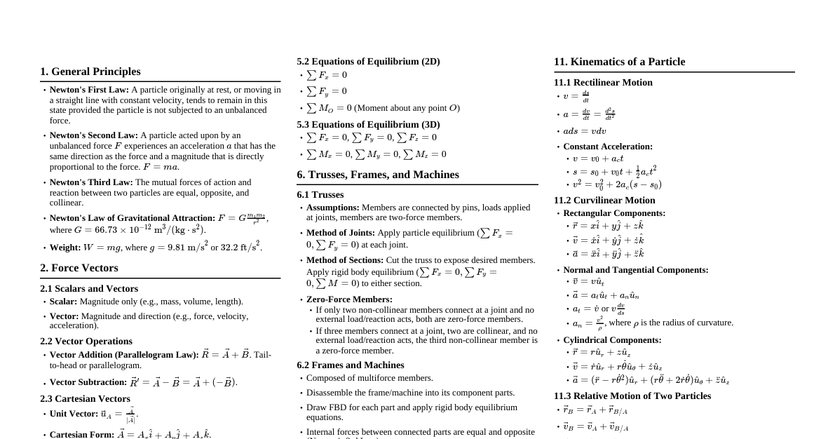
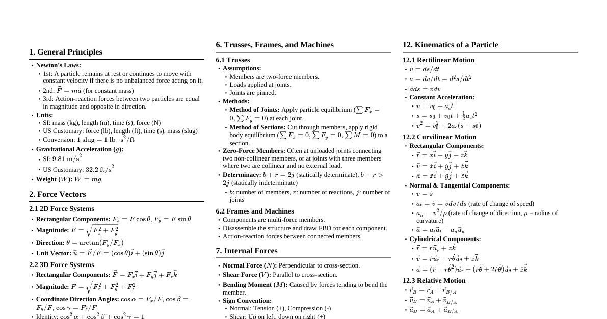
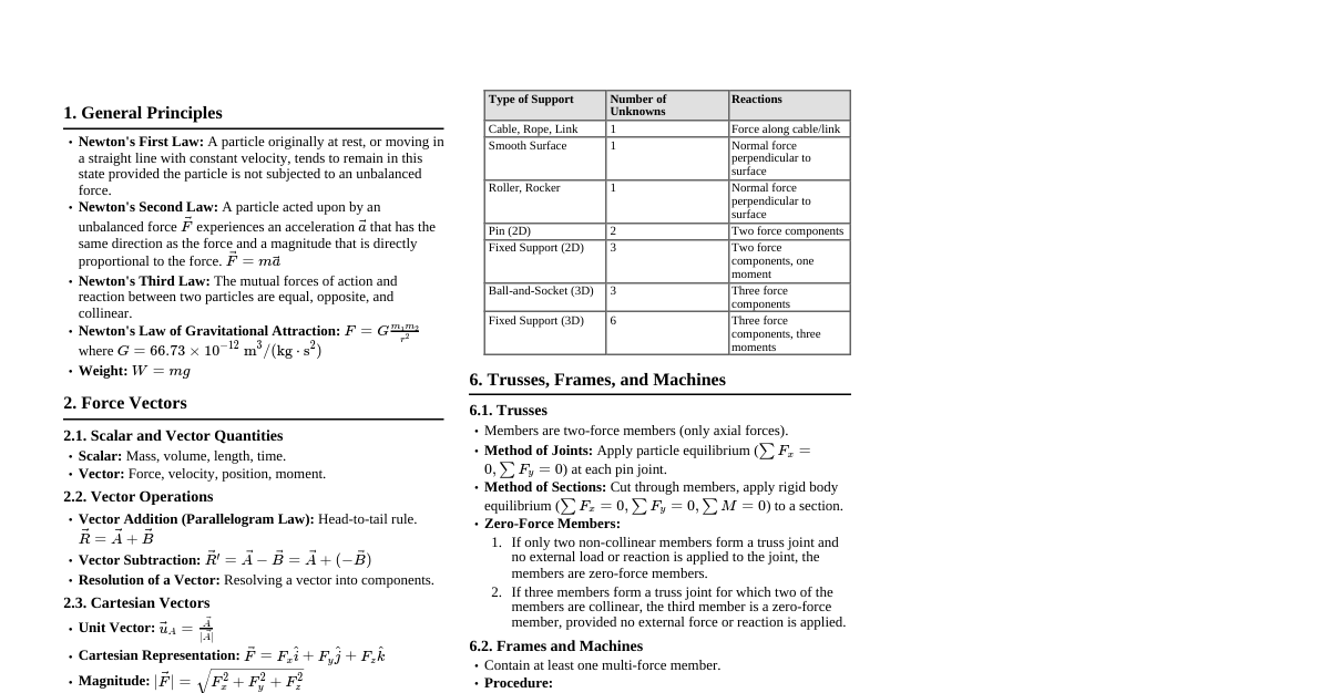
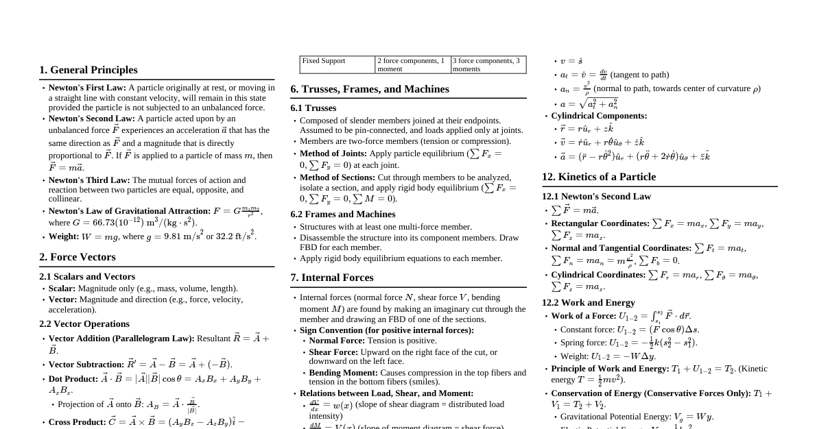
1. General Principles Newton's First Law: A particle originally at rest, or moving in a straight line with constant velocity, tends to remain in this state provided the particle is not subjected to an unbalanced force. Newton's Second Law: A particle acted upon by an unbalanced force $\vec{F}$ experiences an acceleration $\vec{a}$ that has the same direction as the force and a magnitude that is directly proportional to the force. $ \vec{F} = m\vec{a} $ Newton's Third Law: The mutual forces of action and reaction between two particles are equal, opposite, and collinear. Gravitational Law (Newton): $ F = G \frac{m_1 m_2}{r^2} $ where $G = 66.73 \times 10^{-12} \text{ m}^3/(\text{kg} \cdot \text{s}^2)$ Weight: $ W = mg $ where $g = 9.81 \text{ m/s}^2$ or $32.2 \text{ ft/s}^2$ 2. Force Vectors 2.1. Scalar & Vector Quantities Scalar: Mass, volume, length (magnitude only) Vector: Force, velocity, acceleration (magnitude and direction) 2.2. Vector Operations Addition (Parallelogram Law): Head-to-tail method. $\vec{R} = \vec{A} + \vec{B}$ Subtraction: $\vec{R}' = \vec{A} - \vec{B} = \vec{A} + (-\vec{B})$ Resolution into Components: $F_x = F \cos \theta$, $F_y = F \sin \theta$ Magnitude: $F = \sqrt{F_x^2 + F_y^2}$ Direction: $\theta = \tan^{-1}(F_y/F_x)$ 2.3. Cartesian Vectors (3D) Vector Form: $\vec{F} = F_x \hat{i} + F_y \hat{j} + F_z \hat{k}$ Magnitude: $F = \sqrt{F_x^2 + F_y^2 + F_z^2}$ Direction Cosines: $\cos \alpha = F_x/F$, $\cos \beta = F_y/F$, $\cos \gamma = F_z/F$ $\cos^2 \alpha + \cos^2 \beta + \cos^2 \gamma = 1$ Unit Vector: $\hat{u}_F = \frac{\vec{F}}{F} = \cos \alpha \hat{i} + \cos \beta \hat{j} + \cos \gamma \hat{k}$ Position Vector: $\vec{r} = (x_2-x_1)\hat{i} + (y_2-y_1)\hat{j} + (z_2-z_1)\hat{k}$ Force from Position: $\vec{F} = F \left( \frac{\vec{r}}{r} \right)$ 2.4. Dot Product $\vec{A} \cdot \vec{B} = AB \cos \theta$ $\vec{A} \cdot \vec{B} = A_x B_x + A_y B_y + A_z B_z$ Angle between vectors: $\theta = \cos^{-1}\left(\frac{\vec{A} \cdot \vec{B}}{AB}\right)$ Projection of A onto B: $A_B = \vec{A} \cdot \hat{u}_B$ 3. Equilibrium of a Particle Free-Body Diagram (FBD): Critical first step. Isolate particle and show all forces acting ON it. Conditions for Equilibrium: $\sum \vec{F} = 0$ 2D Equations: $\sum F_x = 0$, $\sum F_y = 0$ 3D Equations: $\sum F_x = 0$, $\sum F_y = 0$, $\sum F_z = 0$ Common Supports: Cable: Tension (away from particle) Spring: $F = ks$ (s is deformation) Smooth surface: Normal force (perpendicular to surface) 4. Force System Resultants 4.1. Moment of a Force (Scalar) $M_O = Fd$ (d is perpendicular distance from O to line of action of F) Direction: Right-hand rule (CW is negative, CCW is positive) 4.2. Moment of a Force (Vector) $\vec{M}_O = \vec{r} \times \vec{F}$ (r is position vector from O to any point on line of action of F) Determinant form: $\begin{vmatrix} \hat{i} & \hat{j} & \hat{k} \\ r_x & r_y & r_z \\ F_x & F_y & F_z \end{vmatrix}$ Varignon's Theorem: Moment of a force about a point is equal to the sum of the moments of its components about the same point. $\vec{M}_O = \vec{r} \times (\vec{F}_1 + \vec{F}_2) = (\vec{r} \times \vec{F}_1) + (\vec{r} \times \vec{F}_2)$ 4.3. Moment about an Axis $M_{axis} = \hat{u}_{axis} \cdot (\vec{r} \times \vec{F})$ Scalar projection of moment vector onto the axis unit vector. 4.4. Couple Moment A pair of forces, equal in magnitude, opposite in direction, and parallel. $\vec{M} = \vec{r} \times \vec{F}$ (r is vector from line of action of -F to line of action of F) Magnitude: $M = Fd$ (d is perpendicular distance between forces) A couple moment is a free vector (can be moved anywhere without changing its effect). 4.5. Equivalent Systems Resultant Force: $\vec{F}_R = \sum \vec{F}$ Resultant Couple Moment: $\vec{M}_{R_O} = \sum \vec{M}_O + \sum \vec{M}_{couple}$ A force system can be reduced to a single resultant force $\vec{F}_R$ acting at a point O and a resultant couple moment $\vec{M}_{R_O}$. Wrench (Screw) System: If $\vec{F}_R$ and $\vec{M}_{R_O}$ are parallel. 4.6. Distributed Loading Resultant Force: $F_R = \int w(x) dx$ (area under loading curve) Location of Resultant: $\bar{x} = \frac{\int x w(x) dx}{\int w(x) dx}$ (centroid of the area) 5. Equilibrium of a Rigid Body 5.1. Conditions for Equilibrium $\sum \vec{F} = 0$ (Sum of forces is zero) $\sum \vec{M}_O = 0$ (Sum of moments about any point O is zero) 5.2. 2D Equilibrium Equations $\sum F_x = 0$ $\sum F_y = 0$ $\sum M_O = 0$ Alternative: $\sum F_x = 0$, $\sum M_A = 0$, $\sum M_B = 0$ (A, B not on line perp. to x-axis) Alternative: $\sum M_A = 0$, $\sum M_B = 0$, $\sum M_C = 0$ (A, B, C not collinear) 5.3. 3D Equilibrium Equations $\sum F_x = 0$, $\sum F_y = 0$, $\sum F_z = 0$ $\sum M_x = 0$, $\sum M_y = 0$, $\sum M_z = 0$ 5.4. Supports and Reactions Type of Connection Number of Unknowns Reaction Forces/Moments Cable, Rope, Link 1 Force along cable/link Smooth Surface 1 Normal force $\perp$ surface Roller, Rocker 1 Normal force $\perp$ surface Rough Surface 2 Normal force, Friction force Pin (2D) 2 $F_x$, $F_y$ Fixed Support (2D) 3 $F_x$, $F_y$, $M_z$ Ball-and-Socket (3D) 3 $F_x$, $F_y$, $F_z$ Hinge (3D) 4 or 5 $F_x, F_y, F_z$ and $M_x, M_y$ (if single bearing) Fixed Support (3D) 6 $F_x, F_y, F_z, M_x, M_y, M_z$ 6. Trusses, Frames, and Machines 6.1. Trusses (Pin-connected members, only two-force members) Assumptions: Loads applied at joints, members connected by smooth pins, member weights negligible. Two-Force Member: Member subjected to forces at only two points; forces must be equal, opposite, and collinear. Method of Joints: Draw FBD of entire truss to find external reactions. Draw FBD of each joint. Apply $\sum F_x = 0$, $\sum F_y = 0$ to each joint. Start at a joint with at most two unknown member forces. Zero-Force Members: If only two non-collinear members connect at a joint with no external load, both are zero-force members. If three members connect at a joint, two are collinear, and no external load, the third is a zero-force member. Method of Sections: Draw FBD of entire truss. Cut the truss through members whose forces are desired (max 3 members). Draw FBD of one section. Apply $\sum F_x = 0$, $\sum F_y = 0$, $\sum M_O = 0$. 6.2. Frames and Machines (Multi-force members) Frames: Stationary structures designed to support loads. Machines: Structures containing moving parts, designed to transmit/modify forces. Analysis Procedure: Draw FBD of the entire structure to find external reactions. Disassemble the structure and draw FBD for each part. Apply equilibrium equations ($\sum F = 0, \sum M = 0$) to each part. Remember Newton's 3rd Law for forces between connected parts (equal and opposite). 7. Internal Forces Normal Force (N): Perpendicular to cross-section. Shear Force (V): Tangential to cross-section. Bending Moment (M): Causes bending. Procedure: Find external reactions. Make an imaginary cut through the member at the desired location. Draw FBD of either segment. Apply equilibrium equations to find N, V, M. Sign Convention: (Positive) N: Tension (pulling away) V: Downward on right face, upward on left face (causes CCW rotation) M: Causes compression at top, tension at bottom (smiley face) Relations between Load, Shear, Moment: $\frac{dV}{dx} = -w(x)$ (Slope of shear diagram = negative of distributed load intensity) $\frac{dM}{dx} = V(x)$ (Slope of moment diagram = shear force) $\Delta V = -\int w(x) dx$ (Change in shear = negative area under load curve) $\Delta M = \int V(x) dx$ (Change in moment = area under shear curve) 8. Friction Static Friction: $F_s \le \mu_s N$ $F_s$ is the force of static friction, $\mu_s$ is the coefficient of static friction, $N$ is the normal force. $F_s^{max} = \mu_s N$ (occurs just before motion begins) Kinetic Friction: $F_k = \mu_k N$ $F_k$ is the force of kinetic friction, $\mu_k$ is the coefficient of kinetic friction. $\mu_k Angle of Static Friction: $\tan \phi_s = \mu_s$ Angle of Repose: Maximum angle of inclination for an object on an inclined plane before it slides. $\theta_{max} = \phi_s$. 9. Center of Gravity and Centroid Center of Gravity (CG): Point where the entire weight of a body can be considered to act. $\bar{x} = \frac{\sum \tilde{x} W}{\sum W}$, $\bar{y} = \frac{\sum \tilde{y} W}{\sum W}$, $\bar{z} = \frac{\sum \tilde{z} W}{\sum W}$ For continuous bodies: $\bar{x} = \frac{\int \tilde{x} dW}{\int dW}$, etc. Centroid: Geometric center of an area or volume. (If material is homogeneous, CG coincides with centroid.) Area: $\bar{x} = \frac{\sum \tilde{x} A}{\sum A}$, $\bar{y} = \frac{\sum \tilde{y} A}{\sum A}$ For continuous areas: $\bar{x} = \frac{\int \tilde{x} dA}{\int dA}$, $\bar{y} = \frac{\int \tilde{y} dA}{\int dA}$ Volume: $\bar{x} = \frac{\sum \tilde{x} V}{\sum V}$, etc. Line: $\bar{x} = \frac{\sum \tilde{x} L}{\sum L}$, etc. Theorems of Pappus and Guldinus: Area of Surface of Revolution: $A = \theta \bar{r} L$ (L = length of curve, $\bar{r}$ = distance from axis to centroid of curve, $\theta$ = angle of revolution in radians) Volume of Body of Revolution: $V = \theta \bar{r} A$ (A = area of region, $\bar{r}$ = distance from axis to centroid of area, $\theta$ = angle of revolution in radians) 10. Moments of Inertia 10.1. Area Moments of Inertia $I_x = \int y^2 dA$ $I_y = \int x^2 dA$ Polar Moment of Inertia: $J_O = \int r^2 dA = I_x + I_y$ Radius of Gyration: $k_x = \sqrt{I_x/A}$, $k_y = \sqrt{I_y/A}$, $k_O = \sqrt{J_O/A}$ Parallel-Axis Theorem: $I_x = \bar{I}_x + Ad_y^2$ $I_y = \bar{I}_y + Ad_x^2$ $J_O = \bar{J}_C + Ad^2$ ($\bar{I}$ is moment of inertia about centroidal axis, $d$ is perpendicular distance between parallel axes) 10.2. Mass Moments of Inertia $I = \int r^2 dm$ For a thin plate: $dm = \rho t dA$ ($\rho$ = mass density, $t$ = thickness) Radius of Gyration: $k = \sqrt{I/m}$ Parallel-Axis Theorem: $I = \bar{I} + md^2$