Machine Learning Cheat Sheet

Cheatsheet Content

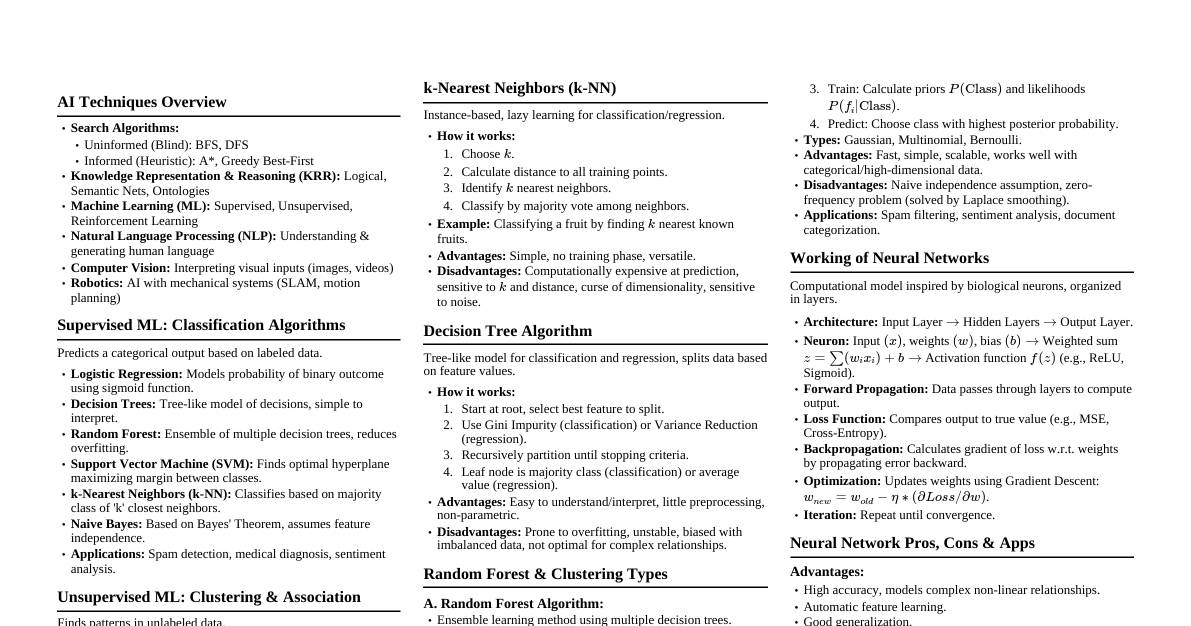
1. Supervised Learning Learns a function from labeled training data. Predicts output for new inputs. 1.1 Regression Predicts a continuous output value. Linear Regression: $y = \theta_0 + \theta_1 x_1 + \dots + \theta_n x_n$ Cost Function (MSE): $J(\theta) = \frac{1}{2m} \sum_{i=1}^m (h_\theta(x^{(i)}) - y^{(i)})^2$ Gradient Descent Update: $\theta_j := \theta_j - \alpha \frac{\partial}{\partial \theta_j} J(\theta)$ Polynomial Regression: Extends linear model with polynomial features. Support Vector Regression (SVR): Finds a function $f(x)$ that deviates from $y$ by at most $\epsilon$. 1.2 Classification Predicts a discrete class label. Logistic Regression: Estimates probability $P(y=1|x;\theta)$ Sigmoid Function: $h_\theta(x) = g(\theta^T x) = \frac{1}{1 + e^{-\theta^T x}}$ Cost Function: $J(\theta) = -\frac{1}{m} \sum_{i=1}^m [y^{(i)} \log(h_\theta(x^{(i)})) + (1-y^{(i)}) \log(1-h_\theta(x^{(i)}))]$ Support Vector Machine (SVM): Finds the hyperplane that best separates classes. Kernel Trick: Maps data into higher-dimensional space for non-linear separation. Common kernels: Linear, Polynomial, RBF (Gaussian). Decision Trees: Tree-like model where each internal node is a test on an attribute, each branch is an outcome of the test, and each leaf node holds a class label. Gini Impurity: $G = 1 - \sum_{k=1}^K p_k^2$ Entropy: $H = -\sum_{k=1}^K p_k \log_2(p_k)$ K-Nearest Neighbors (KNN): Classifies a data point based on the majority class of its $k$ nearest neighbors. Naive Bayes: Probabilistic classifier based on Bayes' Theorem with strong independence assumptions. $P(C|X) = \frac{P(X|C)P(C)}{P(X)}$ 2. Unsupervised Learning Finds hidden patterns or intrinsic structures in unlabeled data. 2.1 Clustering Groups data points into clusters such that points in the same cluster are more similar to each other than to those in other clusters. K-Means: Iteratively assigns data points to $K$ clusters and updates cluster centroids. Objective: Minimize sum of squared distances of points to their assigned cluster centroid. Hierarchical Clustering: Builds a hierarchy of clusters. Agglomerative (bottom-up) or Divisive (top-down). DBSCAN: Density-based spatial clustering of applications with noise. Groups together points that are closely packed together, marking as outliers points that lie alone in low-density regions. 2.2 Dimensionality Reduction Reduces the number of random variables under consideration by obtaining a set of principal variables. Principal Component Analysis (PCA): Transforms data to a new coordinate system such that the greatest variance by any projection of the data comes to lie on the first coordinate (called the first principal component), the second greatest variance on the second coordinate, and so on. t-SNE: t-distributed Stochastic Neighbor Embedding. Non-linear dimensionality reduction technique well-suited for visualizing high-dimensional datasets. 3. Reinforcement Learning Agent learns to make decisions by performing actions in an environment to maximize a cumulative reward. Agent: The learner/decision-maker. Environment: The world the agent interacts with. State ($S$): Current situation of the agent. Action ($A$): Agent's move in a given state. Reward ($R$): Feedback from the environment ($+ve$ for good, $-ve$ for bad). Policy ($\pi$): Strategy that defines the agent's action in each state. $\pi(a|s) = P(A_t=a|S_t=s)$. Value Function ($V(s)$): Expected cumulative reward from state $s$. $V^\pi(s) = E_\pi[\sum_{k=0}^\infty \gamma^k R_{t+k+1} | S_t=s]$. Q-Value Function ($Q(s,a)$): Expected cumulative reward from taking action $a$ in state $s$. $Q^\pi(s,a) = E_\pi[\sum_{k=0}^\infty \gamma^k R_{t+k+1} | S_t=s, A_t=a]$. Bellman Equation: $V(s) = \max_a (R(s,a) + \gamma V(s'))$. Q-Learning: Off-policy algorithm for learning $Q$-values. $Q(S_t, A_t) \leftarrow Q(S_t, A_t) + \alpha [R_{t+1} + \gamma \max_a Q(S_{t+1}, a) - Q(S_t, A_t)]$ 4. Neural Networks & Deep Learning Composed of layers of interconnected nodes (neurons). Perceptron: Simplest neural network, a single neuron for binary classification. Activation Functions: Introduce non-linearity. Sigmoid: $\sigma(z) = \frac{1}{1+e^{-z}}$ ReLU: $max(0, z)$ Softmax: $P(y=k|\mathbf{x}) = \frac{e^{z_k}}{\sum_{j=1}^K e^{z_j}}$ Feedforward Neural Networks (FNN): Information flows in one direction, from input to output. Convolutional Neural Networks (CNN): Specialized for grid-like data (e.g., images). Convolutional Layer: Applies filters to input. Pooling Layer: Reduces spatial dimensions (e.g., Max Pooling). Recurrent Neural Networks (RNN): Designed for sequential data (e.g., text, time series). LSTM (Long Short-Term Memory): Addresses vanishing gradient problem in RNNs. GRU (Gated Recurrent Unit): Simpler variant of LSTM. Backpropagation: Algorithm to train neural networks by computing gradients of the loss function with respect to weights. Optimizers: Adjust learning rate during training. SGD (Stochastic Gradient Descent) Adam (Adaptive Moment Estimation) RMSprop (Root Mean Square Propagation) 5. Model Evaluation Metrics 5.1 Regression Metrics Mean Squared Error (MSE): $\frac{1}{n} \sum_{i=1}^n (y_i - \hat{y}_i)^2$ Root Mean Squared Error (RMSE): $\sqrt{\frac{1}{n} \sum_{i=1}^n (y_i - \hat{y}_i)^2}$ Mean Absolute Error (MAE): $\frac{1}{n} \sum_{i=1}^n |y_i - \hat{y}_i|$ R-squared ($R^2$): $1 - \frac{\sum_{i=1}^n (y_i - \hat{y}_i)^2}{\sum_{i=1}^n (y_i - \bar{y})^2}$ 5.2 Classification Metrics Based on Confusion Matrix: Predicted Positive Predicted Negative Actual Positive True Positive (TP) False Negative (FN) Actual Negative False Positive (FP) True Negative (TN) Accuracy: $\frac{TP + TN}{TP + TN + FP + FN}$ Precision: $\frac{TP}{TP + FP}$ (Positive Predictive Value) Recall (Sensitivity): $\frac{TP}{TP + FN}$ (True Positive Rate) F1-Score: $2 \cdot \frac{Precision \cdot Recall}{Precision + Recall}$ Specificity: $\frac{TN}{TN + FP}$ (True Negative Rate) ROC Curve & AUC: Plots True Positive Rate vs. False Positive Rate. AUC (Area Under Curve) measures overall performance. 5.3 Clustering Metrics Silhouette Score: Measures how similar an object is to its own cluster compared to other clusters. Range $[-1, 1]$. Higher is better. Davies-Bouldin Index: Ratio of within-cluster distances to between-cluster distances. Lower is better. 6. Bias-Variance Trade-off Bias: Error from erroneous assumptions in the learning algorithm (underfitting). Variance: Error from sensitivity to small fluctuations in the training set (overfitting). High Bias, Low Variance: Model is too simple, misses relationships in data. Low Bias, High Variance: Model is too complex, fits noise in training data. Goal: Find a balance between bias and variance. 7. Regularization Techniques to prevent overfitting. L1 Regularization (Lasso): Adds sum of absolute values of coefficients to loss function. Encourages sparsity (some weights become zero for feature selection). Loss + $\lambda \sum |\theta_j|$ L2 Regularization (Ridge): Adds sum of squared values of coefficients to loss function. Shrinks coefficients towards zero. Loss + $\lambda \sum \theta_j^2$ Elastic Net: Combination of L1 and L2. Dropout: Randomly sets a fraction of neuron outputs to zero during training, preventing complex co-adaptations. Early Stopping: Stop training when performance on a validation set starts to degrade. 8. Cross-Validation Technique to evaluate model performance and generalize to unseen data. Hold-out Validation: Split data into training and test sets. K-Fold Cross-Validation: Divide data into $K$ folds. Train on $K-1$ folds and validate on the remaining fold, repeat $K$ times. Average results. Leave-One-Out Cross-Validation (LOOCV): K-Fold where $K=N$ (number of data points).