New sheet - 10/18 09:01
Cheatsheet Content
Linear Algebra: Matrices A matrix is a rectangular array of numbers, symbols, or expressions, arranged in rows and columns. Transpose of a Matrix ($A^T$) The transpose of a matrix $A$ is obtained by interchanging its rows and columns. If $A = [a_{ij}]$, then $A^T = [a_{ji}]$. Example: If $A = \begin{pmatrix} 1 & 2 \\ 3 & 4 \end{pmatrix}$, then $A^T = \begin{pmatrix} 1 & 3 \\ 2 & 4 \end{pmatrix}$. Properties of Transpose Matrix $(A^T)^T = A$ $(A+B)^T = A^T + B^T$ $(kA)^T = kA^T$ (where $k$ is a scalar) $(AB)^T = B^T A^T$ Trace of a Matrix (Tr(A)) The trace of a square matrix is the sum of the elements on its main diagonal. For $A = [a_{ij}]$, $Tr(A) = \sum_{i=1}^n a_{ii}$. Example: For $A = \begin{pmatrix} 1 & 2 & 3 \\ 4 & 5 & 6 \\ 7 & 8 & 9 \end{pmatrix}$, $Tr(A) = 1+5+9=15$. Types of Matrices Square Matrix: Number of rows = Number of columns ($n \times n$). Identity Matrix ($I$ or $I_n$): A square matrix with ones on the main diagonal and zeros elsewhere. $$ I_3 = \begin{pmatrix} 1 & 0 & 0 \\ 0 & 1 & 0 \\ 0 & 0 & 1 \end{pmatrix} $$ Zero Matrix ($0$): All elements are zero. Diagonal Matrix: A square matrix where all non-diagonal elements are zero. Scalar Matrix: A diagonal matrix where all diagonal elements are equal ($kI$). Symmetric Matrix: $A^T = A$. ($a_{ij} = a_{ji}$) Skew-Symmetric Matrix: $A^T = -A$. ($a_{ij} = -a_{ji}$, diagonal elements are 0). Orthogonal Matrix: A square matrix $A$ such that $A^T A = A A^T = I$. Implies $A^{-1} = A^T$. Idempotent Matrix: $A^2 = A$. Nilpotent Matrix: $A^k = 0$ for some positive integer $k$. Involutory Matrix: $A^2 = I$. Orthonormal Vectors A set of vectors $\{v_1, v_2, \dots, v_k\}$ is orthonormal if they are all unit vectors and are mutually orthogonal. Unit vector: $||v_i|| = 1$ Mutually orthogonal: $v_i \cdot v_j = 0$ for $i \neq j$ This can be summarized as $v_i^T v_j = \delta_{ij}$ (Kronecker delta). LU Decomposition Factorizes a matrix $A$ into a product of a lower triangular matrix $L$ and an upper triangular matrix $U$, i.e., $A = LU$. Used to solve systems of linear equations efficiently, calculate determinants, and invert matrices. Cholesky Decomposition For a symmetric, positive-definite matrix $A$, it can be decomposed as $A = LL^T$, where $L$ is a lower triangular matrix with positive diagonal entries. Determinant of a Matrix A scalar value that can be computed from the elements of a square matrix. It characterizes certain properties of the matrix and the linear transformation it represents. Properties of Determinants $\det(I) = 1$ $\det(A^T) = \det(A)$ $\det(AB) = \det(A) \det(B)$ $\det(kA) = k^n \det(A)$ for an $n \times n$ matrix $A$. If two rows (or columns) are identical, $\det(A) = 0$. If a row (or column) is all zeros, $\det(A) = 0$. If a matrix has linearly dependent rows/columns, $\det(A) = 0$. Swapping two rows (or columns) changes the sign of the determinant. Adding a multiple of one row (or column) to another row (or column) does not change the determinant. For an upper/lower triangular matrix, the determinant is the product of its diagonal elements. Methods to Find Determinants $2 \times 2$ Matrix: $\det \begin{pmatrix} a & b \\ c & d \end{pmatrix} = ad - bc$. Cofactor Expansion: For an $n \times n$ matrix, $\det(A) = \sum_{j=1}^n (-1)^{i+j} a_{ij} M_{ij}$ (along row $i$) or $\sum_{i=1}^n (-1)^{i+j} a_{ij} M_{ij}$ (along column $j$). $M_{ij}$ is the determinant of the submatrix obtained by deleting row $i$ and column $j$. Row Reduction (Gaussian Elimination): Reduce the matrix to an upper triangular form using elementary row operations, keeping track of row swaps (sign changes) and scalar multiplications (factor out). The determinant is then the product of the diagonal entries, adjusted by the accumulated factors and signs. Linear Dependency and Determinants A set of vectors $\{v_1, \dots, v_n\}$ is linearly dependent if and only if the determinant of the matrix formed by these vectors as columns (or rows) is zero. Example: Vectors $\begin{pmatrix} 1 \\ 2 \end{pmatrix}$ and $\begin{pmatrix} 2 \\ 4 \end{pmatrix}$ are linearly dependent because $\det \begin{pmatrix} 1 & 2 \\ 2 & 4 \end{pmatrix} = 4-4=0$. Elementary Transformations Operations that can be performed on rows (or columns) of a matrix: Swapping two rows ($R_i \leftrightarrow R_j$). Changes determinant sign. Multiplying a row by a non-zero scalar ($kR_i \rightarrow R_i$). Multiplies determinant by $k$. Adding a multiple of one row to another row ($R_i + kR_j \rightarrow R_i$). No change to determinant. Partitioned Matrices (Block Matrices) A matrix whose entries are themselves matrices (blocks). If $M = \begin{pmatrix} A & B \\ C & D \end{pmatrix}$ where $A, B, C, D$ are matrices. If $A$ is invertible, $\det(M) = \det(A) \det(D - CA^{-1}B)$. If $M = \begin{pmatrix} A & 0 \\ C & D \end{pmatrix}$ or $M = \begin{pmatrix} A & B \\ 0 & D \end{pmatrix}$ (block triangular), then $\det(M) = \det(A) \det(D)$. Inverse of a Matrix ($A^{-1}$) For a square matrix $A$, its inverse $A^{-1}$ satisfies $AA^{-1} = A^{-1}A = I$. A matrix is invertible if and only if $\det(A) \neq 0$. Formula: $A^{-1} = \frac{1}{\det(A)} \text{adj}(A)$, where $\text{adj}(A)$ is the adjugate matrix (transpose of the cofactor matrix). Shortcut for $2 \times 2$ Inverse If $A = \begin{pmatrix} a & b \\ c & d \end{pmatrix}$, then $A^{-1} = \frac{1}{ad-bc} \begin{pmatrix} d & -b \\ -c & a \end{pmatrix}$. Rank of a Matrix The rank of a matrix $A$, denoted $rank(A)$, is the maximum number of linearly independent row vectors or column vectors in the matrix. It is also the dimension of the column space (image) or row space of the matrix. Finding Rank Using Minors: The rank of a matrix is the order of the largest non-zero minor (determinant of a square submatrix). Using Linear Dependency: Find the maximum number of linearly independent rows/columns. Using Echelon Form (Gaussian Elimination): The rank of a matrix is the number of non-zero rows in its row echelon form or reduced row echelon form. Example: For $A = \begin{pmatrix} 1 & 2 & 3 \\ 0 & 1 & 4 \\ 0 & 0 & 0 \end{pmatrix}$ (already in echelon form), $rank(A)=2$ because there are two non-zero rows. Properties of Rank $rank(A) \le \min(m, n)$ for an $m \times n$ matrix. $rank(A) = rank(A^T)$. $rank(AB) \le \min(rank(A), rank(B))$. $rank(A+B) \le rank(A) + rank(B)$. If $A$ is an $n \times n$ matrix, $rank(A)=n \iff \det(A) \neq 0 \iff A$ is invertible. Linear System of Equations A set of linear equations involving the same variables. Generally written as $Ax=b$. Classification of Linear Systems Linear System Consistent Inconsistent Unique Solution Infinite Solutions Consistent: Has at least one solution (unique or infinite). Inconsistent: Has no solution. Homogeneous vs. Non-Homogeneous Systems Homogeneous System: $Ax = 0$. Always consistent (has at least the trivial solution $x=0$). Unique solution: $x=0$ (trivial solution) if $rank(A) = n$ (number of variables). Infinite solutions: If $rank(A) Non-Homogeneous System: $Ax = B$ ($B \neq 0$). Consistent if $rank(A) = rank([A|B])$ (Augmented Matrix). Unique solution if $rank(A) = rank([A|B]) = n$. Infinite solutions if $rank(A) = rank([A|B]) Inconsistent if $rank(A) \neq rank([A|B])$. Augmented Matrix For $Ax=B$, the augmented matrix is $[A|B]$. It combines the coefficient matrix $A$ and the constant vector $B$. Example: For $x+2y=5$, $3x+4y=6$, the augmented matrix is $\begin{pmatrix} 1 & 2 & | & 5 \\ 3 & 4 & | & 6 \end{pmatrix}$. Underdetermined System A system where the number of equations is less than the number of variables ($m Null Space and Nullity Null Space ($N(A)$): The set of all solutions to the homogeneous equation $Ax=0$. It is a subspace of the domain. Nullity: The dimension of the null space, $nullity(A) = \dim(N(A))$. Rank-Nullity Theorem: For an $m \times n$ matrix $A$, $rank(A) + nullity(A) = n$ (number of columns/variables). For $Ax=0$, the number of independent solutions is $n - rank(A)$. Eigenvalues and Eigenvectors For a square matrix $A$, an eigenvector $v$ is a non-zero vector that, when multiplied by $A$, only changes magnitude, not direction. The scaling factor is the eigenvalue $\lambda$. Equation: $Av = \lambda v$. Equation of Eigenvalues $(A - \lambda I)v = 0$. For non-trivial solutions ($v \neq 0$), the matrix $(A - \lambda I)$ must be singular, meaning its determinant is zero: $\det(A - \lambda I) = 0$. This is the characteristic equation. Properties of Eigenvalues The sum of eigenvalues is equal to the trace of the matrix: $\sum \lambda_i = Tr(A)$. The product of eigenvalues is equal to the determinant of the matrix: $\prod \lambda_i = \det(A)$. If $\lambda$ is an eigenvalue of $A$, then $\lambda^k$ is an eigenvalue of $A^k$. If $\lambda$ is an eigenvalue of $A$ and $A$ is invertible, then $1/\lambda$ is an eigenvalue of $A^{-1}$. Eigenvalues of a symmetric matrix are always real. Eigenvectors corresponding to distinct eigenvalues are linearly independent. Cayley-Hamilton Theorem Every square matrix satisfies its own characteristic equation. If the characteristic equation is $P(\lambda) = a_n \lambda^n + \dots + a_1 \lambda + a_0 = 0$, then $P(A) = a_n A^n + \dots + a_1 A + a_0 I = 0$. Useful for finding powers of a matrix or its inverse. Diagonalization of Matrices A square matrix $A$ is diagonalizable if there exists an invertible matrix $P$ such that $P^{-1}AP = D$, where $D$ is a diagonal matrix. The diagonal entries of $D$ are the eigenvalues of $A$, and the columns of $P$ are the corresponding eigenvectors. A matrix is diagonalizable if and only if it has $n$ linearly independent eigenvectors. Basics of Vector Space A set $V$ of vectors, together with two operations (vector addition and scalar multiplication), that satisfy eight axioms. Key concepts include: Span: The set of all linear combinations of a given set of vectors. Linear Independence: A set of vectors where no vector can be written as a linear combination of the others. Basis: A linearly independent set of vectors that spans the entire vector space. Dimension: The number of vectors in any basis for the vector space. Vector Calculus Calculus extended to vector fields and functions of multiple variables. Scalar Triple Product For three vectors $a, b, c$, the scalar triple product is $a \cdot (b \times c)$. Geometrically, it represents the volume of the parallelepiped formed by the three vectors. It can be calculated as the determinant of the matrix formed by the vectors: $$ a \cdot (b \times c) = \det \begin{pmatrix} a_1 & a_2 & a_3 \\ b_1 & b_2 & b_3 \\ c_1 & c_2 & c_3 \end{pmatrix} $$ Properties: $a \cdot (b \times c) = b \cdot (c \times a) = c \cdot (a \times b)$. If $a, b, c$ are coplanar, then $a \cdot (b \times c) = 0$. Vector Triple Product For three vectors $a, b, c$, the vector triple product is $a \times (b \times c)$. Formula: $a \times (b \times c) = (a \cdot c)b - (a \cdot b)c$. (BAC-CAB rule) Vector Differential Operator ($\nabla$) Also known as "del" or "nabla". In Cartesian coordinates, $\nabla = \frac{\partial}{\partial x} \mathbf{i} + \frac{\partial}{\partial y} \mathbf{j} + \frac{\partial}{\partial z} \mathbf{k}$. Gradient ($\nabla \phi$): For a scalar field $\phi(x,y,z)$, $\nabla \phi$ is a vector field pointing in the direction of the greatest rate of increase of $\phi$. Divergence ($\nabla \cdot F$): For a vector field $F = P\mathbf{i} + Q\mathbf{j} + R\mathbf{k}$, $\nabla \cdot F = \frac{\partial P}{\partial x} + \frac{\partial Q}{\partial y} + \frac{\partial R}{\partial z}$. It measures the outward flux per unit volume. Curl ($\nabla \times F$): For a vector field $F = P\mathbf{i} + Q\mathbf{j} + R\mathbf{k}$, $$ \nabla \times F = \det \begin{pmatrix} \mathbf{i} & \mathbf{j} & \mathbf{k} \\ \frac{\partial}{\partial x} & \frac{\partial}{\partial y} & \frac{\partial}{\partial z} \\ P & Q & R \end{pmatrix} $$ It measures the rotation or circulation of the vector field. Unit Normal Vector For a surface defined by $\phi(x,y,z) = c$, the unit normal vector $\mathbf{n}$ is given by $\mathbf{n} = \frac{\nabla \phi}{||\nabla \phi||}$. Directional Derivative The rate of change of a scalar function $\phi$ in the direction of a unit vector $\mathbf{u}$ is given by $D_{\mathbf{u}} \phi = \nabla \phi \cdot \mathbf{u}$. Vector Identities $\nabla \cdot (\nabla \phi) = \nabla^2 \phi$ (Laplacian of $\phi$) $\nabla \times (\nabla \phi) = 0$ (Curl of a gradient is zero) $\nabla \cdot (\nabla \times F) = 0$ (Divergence of a curl is zero) $\nabla \times (\nabla \times F) = \nabla(\nabla \cdot F) - \nabla^2 F$ Line Integrals Integrals of a function along a curve. Given a vector field $F$ and a curve $C$ parameterized by $r(t)$, $a \le t \le b$: Line integral of a scalar function $f$ with respect to arc length: $\int_C f(x,y,z) ds = \int_a^b f(r(t)) ||r'(t)|| dt$. Line integral of a vector field $F$: $\int_C F \cdot dr = \int_a^b F(r(t)) \cdot r'(t) dt$. If $F$ is conservative, i.e., $F = \nabla \phi$, then $\int_C F \cdot dr = \phi(B) - \phi(A)$ (path independent), where $A$ and $B$ are the start and end points of $C$. Vector Integral Theorems Green's Theorem: Relates a line integral around a simple closed curve $C$ in the plane to a double integral over the region $D$ bounded by $C$. $$ \oint_C (P dx + Q dy) = \iint_D \left( \frac{\partial Q}{\partial x} - \frac{\partial P}{\partial y} \right) dA $$ Stokes' Theorem: Relates a line integral around a closed curve $C$ (boundary of a surface $S$) to a surface integral over $S$. $$ \oint_C F \cdot dr = \iint_S (\nabla \times F) \cdot dS $$ Gauss's Divergence Theorem: Relates the flux of a vector field $F$ across a closed surface $S$ (boundary of a solid region $E$) to a triple integral over $E$. $$ \iint_S F \cdot dS = \iiint_E (\nabla \cdot F) dV $$ Fourier Series A Fourier series is an expansion of a periodic function into a sum of sines and cosines. General Formula for a function $f(x)$ with period $2L$ $$ f(x) = a_0 + \sum_{n=1}^\infty (a_n \cos(\frac{n\pi x}{L}) + b_n \sin(\frac{n\pi x}{L})) $$ Where the coefficients are given by: $a_0 = \frac{1}{2L} \int_{-L}^{L} f(x) dx$ $a_n = \frac{1}{L} \int_{-L}^{L} f(x) \cos(\frac{n\pi x}{L}) dx$ $b_n = \frac{1}{L} \int_{-L}^{L} f(x) \sin(\frac{n\pi x}{L}) dx$ Cases in Fourier Series Even Function: If $f(-x) = f(x)$, then $b_n = 0$. The series contains only cosine terms and $a_0$. $$ a_0 = \frac{1}{L} \int_{0}^{L} f(x) dx, \quad a_n = \frac{2}{L} \int_{0}^{L} f(x) \cos(\frac{n\pi x}{L}) dx $$ Odd Function: If $f(-x) = -f(x)$, then $a_n = 0$. The series contains only sine terms. $$ b_n = \frac{2}{L} \int_{0}^{L} f(x) \sin(\frac{n\pi x}{L}) dx $$ Half-Range Fourier Series Used to represent a function defined on an interval $(0, L)$ as either an even or an odd function with period $2L$. Half-Range Cosine Series: Extend $f(x)$ as an even function. Coefficients are $a_0, a_n$ as for even functions. Half-Range Sine Series: Extend $f(x)$ as an odd function. Coefficients are $b_n$ as for odd functions. Convergence of Fourier Series (Dirichlet Conditions) If $f(x)$ is periodic with period $2L$ and satisfies the following conditions: $f(x)$ has a finite number of discontinuities in any one period. $f(x)$ has a finite number of maxima and minima in any one period. $f(x)$ is absolutely integrable over one period ($\int_{-L}^L |f(x)| dx Then the Fourier series converges to: $f(x)$ at points where $f(x)$ is continuous. $\frac{f(x^+) + f(x^-)}{2}$ at points where $f(x)$ has a jump discontinuity. Differential Equations An equation involving an unknown function and its derivatives. Types of Differential Equations Ordinary Differential Equation (ODE): Involves derivatives with respect to a single independent variable. Partial Differential Equation (PDE): Involves derivatives with respect to multiple independent variables. Order: The order of the highest derivative in the equation. Degree: The exponent of the highest order derivative after the equation has been rationalized (cleared of fractional powers of derivatives). Linear: The dependent variable and its derivatives appear only to the first power and are not multiplied together. Non-linear: Not linear. First Order Equations Variable Separable: Can be written as $g(y) dy = f(x) dx$. Integrate both sides. Homogeneous: Can be written as $\frac{dy}{dx} = f(\frac{y}{x})$. Substitute $y=vx$, so $\frac{dy}{dx} = v + x\frac{dv}{dx}$. Exact Differential Equations: $M(x,y)dx + N(x,y)dy = 0$ is exact if $\frac{\partial M}{\partial y} = \frac{\partial N}{\partial x}$. The solution is $F(x,y) = C$ where $\frac{\partial F}{\partial x} = M$ and $\frac{\partial F}{\partial y} = N$. Integrating Factor: If not exact, sometimes multiplying by an integrating factor $\mu(x,y)$ makes it exact. If $\frac{1}{N}(\frac{\partial M}{\partial y} - \frac{\partial N}{\partial x})$ is a function of $x$ only, say $f(x)$, then $\mu(x) = e^{\int f(x)dx}$. If $\frac{1}{M}(\frac{\partial N}{\partial x} - \frac{\partial M}{\partial y})$ is a function of $y$ only, say $g(y)$, then $\mu(y) = e^{\int g(y)dy}$. Linear First Order ODE: $\frac{dy}{dx} + P(x)y = Q(x)$. Integrating Factor: $IF = e^{\int P(x)dx}$. Solution: $y \cdot IF = \int Q(x) \cdot IF dx + C$. Bernoulli's Equation: $\frac{dy}{dx} + P(x)y = Q(x)y^n$. Substitute $v = y^{1-n}$. Then $\frac{dv}{dx} = (1-n)y^{-n}\frac{dy}{dx}$. This transforms it into a linear first-order ODE in terms of $v$. Second Order Linear Differential Equations with Constant Coefficients $ay'' + by' + cy = F(x)$. General solution $y(x) = y_c(x) + y_p(x)$, where $y_c$ is the complementary solution (solution to $ay''+by'+cy=0$) and $y_p$ is the particular solution. Complementary Solution ($y_c$) Solve the characteristic equation $ar^2 + br + c = 0$. Distinct Real Roots ($r_1, r_2$): $y_c = C_1 e^{r_1 x} + C_2 e^{r_2 x}$. Repeated Real Roots ($r_1 = r_2 = r$): $y_c = C_1 e^{rx} + C_2 x e^{rx}$. Complex Conjugate Roots ($r = \alpha \pm i\beta$): $y_c = e^{\alpha x}(C_1 \cos(\beta x) + C_2 \sin(\beta x))$. Particular Solution ($y_p$) Methods: Undetermined Coefficients (for specific $F(x)$ forms) or Variation of Parameters. Second Order Linear Differential Equations with Variable Coefficients $P(x)y'' + Q(x)y' + R(x)y = F(x)$. (e.g., Euler-Cauchy Equation) Wronskian ($W(y_1, y_2)$) For two solutions $y_1, y_2$ of $y''+p(x)y'+q(x)y=0$, the Wronskian is $W(y_1, y_2) = \det \begin{pmatrix} y_1 & y_2 \\ y_1' & y_2' \end{pmatrix} = y_1 y_2' - y_2 y_1'$. $y_1, y_2$ are linearly independent if and only if $W(y_1, y_2) \neq 0$. Method of Variation of Parameters For $y''+p(x)y'+q(x)y=f(x)$, if $y_1, y_2$ are linearly independent solutions to the homogeneous equation, then $y_p = u_1 y_1 + u_2 y_2$, where: $u_1 = -\int \frac{y_2 f(x)}{W(y_1, y_2)} dx$ $u_2 = \int \frac{y_1 f(x)}{W(y_1, y_2)} dx$ Higher Order Differential Equations (Constant Coefficients) Similar to 2nd order, solve characteristic equation $a_n r^n + \dots + a_1 r + a_0 = 0$. Distinct Real Roots: $C_1 e^{r_1 x} + C_2 e^{r_2 x} + \dots$ Repeated Real Roots ($r$ repeated $k$ times): $(C_1 + C_2 x + \dots + C_k x^{k-1})e^{rx}$. Complex Conjugate Roots: For each pair $\alpha \pm i\beta$ repeated $k$ times, contributions like $e^{\alpha x}[(C_1 + C_2 x + \dots) \cos(\beta x) + (D_1 + D_2 x + \dots) \sin(\beta x)]$. Euler-Cauchy Differential Equations $ax^2y'' + bxy' + cy = F(x)$. Homogeneous solution: Assume $y = x^m$. Substitute into the homogeneous equation to get an indicial equation for $m$. Distinct Real Roots ($m_1, m_2$): $y_c = C_1 x^{m_1} + C_2 x^{m_2}$. Repeated Real Roots ($m_1 = m_2 = m$): $y_c = C_1 x^m + C_2 x^m \ln|x|$. Complex Conjugate Roots ($m = \alpha \pm i\beta$): $y_c = x^\alpha[C_1 \cos(\beta \ln|x|) + C_2 \sin(\beta \ln|x|)]$. Complex Variables Numbers of the form $z = x + iy$, where $i = \sqrt{-1}$. Amplitude and Polar Form For $z = x+iy$: Modulus (Magnitude): $|z| = r = \sqrt{x^2 + y^2}$. Argument (Angle): $\theta = \arg(z) = \tan^{-1}(\frac{y}{x})$. The principal argument is usually in $(-\pi, \pi]$. Polar Form: $z = r(\cos\theta + i\sin\theta) = re^{i\theta}$. Complex Functions A function $f(z)$ where $z$ is a complex variable. Can be written as $f(z) = u(x,y) + iv(x,y)$, where $u$ and $v$ are real-valued functions of two real variables $x$ and $y$. Analytic Function A complex function $f(z)$ is analytic (or holomorphic) at a point $z_0$ if it is differentiable not only at $z_0$ but also at every point in some neighborhood of $z_0$. Entire Function: A function that is analytic everywhere in the complex plane (e.g., $e^z, \sin z, z^n$). Singular Point: A point where $f(z)$ is not analytic. Cauchy-Riemann Equations A necessary condition for $f(z) = u(x,y) + iv(x,y)$ to be analytic is that its partial derivatives satisfy: $\frac{\partial u}{\partial x} = \frac{\partial v}{\partial y}$ and $\frac{\partial u}{\partial y} = -\frac{\partial v}{\partial x}$. If these conditions hold and the partial derivatives are continuous, then $f(z)$ is analytic. Milne-Thompson Method Used to find an analytic function $f(z)=u+iv$ if either $u(x,y)$ or $v(x,y)$ is given. If $u(x,y)$ is given: 1. Find $\frac{\partial u}{\partial x}$ and $\frac{\partial u}{\partial y}$. 2. Let $\phi_1(x,y) = \frac{\partial u}{\partial x}$ and $\phi_2(x,y) = \frac{\partial u}{\partial y}$. 3. Substitute $x=z, y=0$ into $\phi_1$ and $\phi_2$ to get $\phi_1(z,0)$ and $\phi_2(z,0)$. 4. $f(z) = \int [\phi_1(z,0) - i\phi_2(z,0)] dz + C$. If $v(x,y)$ is given: 1. Find $\frac{\partial v}{\partial x}$ and $\frac{\partial v}{\partial y}$. 2. Let $\psi_1(x,y) = \frac{\partial v}{\partial x}$ and $\psi_2(x,y) = \frac{\partial v}{\partial y}$. 3. Substitute $x=z, y=0$ into $\psi_1$ and $\psi_2$ to get $\psi_1(z,0)$ and $\psi_2(z,0)$. 4. $f(z) = \int [\psi_2(z,0) + i\psi_1(z,0)] dz + C$. Power Series An infinite series of the form $\sum_{n=0}^\infty a_n (z-z_0)^n$. Taylor Series: If $f(z)$ is analytic at $z_0$, then $f(z) = \sum_{n=0}^\infty \frac{f^{(n)}(z_0)}{n!} (z-z_0)^n$. Laurent Series An extension of the Taylor series for functions that are analytic in an annulus (ring-shaped region) but may have singularities inside the inner circle. $$ f(z) = \sum_{n=-\infty}^\infty a_n (z-z_0)^n = \sum_{n=0}^\infty a_n (z-z_0)^n + \sum_{n=1}^\infty \frac{b_n}{(z-z_0)^n} $$ The coefficients are given by $a_n = \frac{1}{2\pi i} \oint_C \frac{f(\zeta)}{(\zeta-z_0)^{n+1}} d\zeta$, where $C$ is a contour in the annulus. The second sum is called the principal part of the Laurent series. Types of Isolated Singularities If $z_0$ is an isolated singular point of $f(z)$: Removable Singularity: The principal part of the Laurent series about $z_0$ contains no terms (e.g., $\frac{\sin z}{z}$ at $z=0$). Pole of Order $m$: The principal part contains a finite number of terms, with the highest power being $\frac{b_m}{(z-z_0)^m}$ and $b_m \neq 0$. If $m=1$, it's a simple pole. (e.g., $\frac{1}{z^2}$ at $z=0$ is a pole of order 2). Essential Singularity: The principal part contains infinitely many terms (e.g., $e^{1/z}$ at $z=0$). Residue of $f(z)$ at a Pole The residue of $f(z)$ at an isolated singular point $z_0$, denoted $\text{Res}(f, z_0)$, is the coefficient $b_1$ of the term $\frac{1}{z-z_0}$ in the Laurent series expansion. For a simple pole ($m=1$): $\text{Res}(f, z_0) = \lim_{z \to z_0} (z-z_0)f(z)$. For a pole of order $m$: $\text{Res}(f, z_0) = \frac{1}{(m-1)!} \lim_{z \to z_0} \frac{d^{m-1}}{dz^{m-1}} [(z-z_0)^m f(z)]$. Cauchy's Residue Theorem If $f(z)$ is analytic inside and on a simple closed contour $C$, except for a finite number of isolated singularities $z_1, z_2, \dots, z_k$ inside $C$, then: $$ \oint_C f(z) dz = 2\pi i \sum_{j=1}^k \text{Res}(f, z_j) $$ Numerical Methods: Solution of Non-Linear Equations Methods to find roots of an equation $f(x)=0$ where $f(x)$ is non-linear. Bisection Method Requires an interval $[a, b]$ such that $f(a)$ and $f(b)$ have opposite signs (guarantees a root within the interval). 1. Find midpoint $c = (a+b)/2$. 2. If $f(c)=0$, then $c$ is the root. 3. If $f(a)f(c) Newton-Raphson Method Uses the tangent line to approximate the root. Requires the derivative $f'(x)$. $$ x_{n+1} = x_n - \frac{f(x_n)}{f'(x_n)} $$ Starts with an initial guess $x_0$. Fast convergence (quadratic) if $x_0$ is close to the root, but may diverge if $f'(x_n)$ is close to zero or $x_0$ is far from the root. Secant Method Similar to Newton-Raphson but approximates the derivative using two previous points, avoiding explicit calculation of $f'(x)$. $$ x_{n+1} = x_n - f(x_n) \frac{x_n - x_{n-1}}{f(x_n) - f(x_{n-1})} $$ Requires two initial guesses $x_0, x_1$. Convergence is superlinear, faster than bisection but slower than Newton-Raphson. No guarantee of convergence. Regula Falsi (False Position) Method Similar to Bisection, but instead of taking the midpoint, it uses the x-intercept of the secant line connecting $(a, f(a))$ and $(b, f(b))$. $$ c = a - \frac{f(a)(b-a)}{f(b)-f(a)} $$ Guaranteed to converge, usually faster than bisection, but one endpoint tends to stay fixed, leading to slower convergence in some cases.