Statistical Inference

Cheatsheet Content

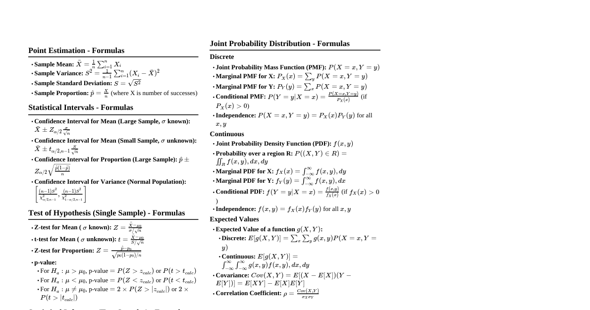
### Point Estimation - **Concept:** Using a single statistic (e.g., sample mean $\bar{X}$) to estimate a population parameter (e.g., population mean $\mu$). - **Estimator Properties:** - **Unbiased:** $E[\hat{\theta}] = \theta$ (expected value of estimator equals true parameter). - **Efficient:** Smallest variance among unbiased estimators. - **Consistent:** As sample size $n \to \infty$, $\hat{\theta} \to \theta$. - **Common Estimators:** - Population Mean $\mu$: Sample Mean $\bar{X} = \frac{1}{n}\sum_{i=1}^n X_i$ - Population Variance $\sigma^2$: Sample Variance $S^2 = \frac{1}{n-1}\sum_{i=1}^n (X_i - \bar{X})^2$ - Population Proportion $p$: Sample Proportion $\hat{p} = \frac{X}{n}$ (where X is number of successes) - **Solving:** Directly compute the sample statistic from given data. - *Example:* If sample data is [10, 12, 11, 9, 13], then $\bar{X} = (10+12+11+9+13)/5 = 11$. This is the point estimate for $\mu$. ### Statistical Intervals (Confidence Intervals) - **Concept:** An interval estimate for a population parameter, constructed such that it contains the true parameter with a certain probability (confidence level). - **General Form:** Point Estimate $\pm$ (Critical Value $\times$ Standard Error) - **Confidence Level $(1-\alpha)$:** Probability that the interval contains the true parameter. Common levels: 90%, 95%, 99%. - **Interpretation:** A 95% CI for $\mu$ means that if we were to construct many such intervals from repeated samples, 95% of them would contain the true $\mu$. It does NOT mean there's a 95% chance the true $\mu$ is in *this specific* interval. #### Confidence Interval for $\mu$ (Population Mean) - **Known $\sigma$ (Population Standard Deviation):** $$ \bar{X} \pm z_{\alpha/2} \frac{\sigma}{\sqrt{n}} $$ - $z_{\alpha/2}$ is the critical value from the standard normal distribution. - **Unknown $\sigma$ (Sample Standard Deviation $S$ used):** $$ \bar{X} \pm t_{\alpha/2, n-1} \frac{S}{\sqrt{n}} $$ - $t_{\alpha/2, n-1}$ is the critical value from the t-distribution with $n-1$ degrees of freedom. #### Confidence Interval for $p$ (Population Proportion) - **Formula:** $$ \hat{p} \pm z_{\alpha/2} \sqrt{\frac{\hat{p}(1-\hat{p})}{n}} $$ - Requires $n\hat{p} \ge 5$ and $n(1-\hat{p}) \ge 5$ for normal approximation. - **Solving Steps:** 1. Identify the parameter to be estimated ($\mu$ or $p$). 2. Determine the point estimate ($\bar{X}$ or $\hat{p}$). 3. Choose confidence level $(1-\alpha)$ and find critical value ($z_{\alpha/2}$ or $t_{\alpha/2, n-1}$). 4. Calculate the standard error of the estimate. 5. Construct the interval. - *Example (known $\sigma$):* Sample mean $\bar{X}=50$, $\sigma=10$, $n=100$. For a 95% CI, $z_{0.025}=1.96$. $$ 50 \pm 1.96 \frac{10}{\sqrt{100}} = 50 \pm 1.96(1) = (48.04, 51.96) $$ ### Test of Hypothesis in Single Sample - **Concept (More on Concept):** A formal procedure to evaluate a claim (hypothesis) about a population parameter using sample data. - **Key Components:** 1. **Null Hypothesis ($H_0$):** A statement of "no effect" or "no difference." Always contains an equality ($=, \le, \ge$). 2. **Alternative Hypothesis ($H_1$ or $H_a$):** The claim we are trying to find evidence for. Contradicts $H_0$ (e.g., $\ne, $). 3. **Test Statistic:** A value calculated from sample data, used to assess how consistent the data is with $H_0$. 4. **P-value:** The probability of observing a test statistic as extreme as, or more extreme than, the one calculated, *assuming $H_0$ is true*. A small p-value suggests evidence against $H_0$. 5. **Significance Level ($\alpha$):** A pre-determined threshold (e.g., 0.05). If p-value $\le \alpha$, we reject $H_0$. 6. **Decision:** Reject $H_0$ or Fail to Reject $H_0$. 7. **Conclusion:** State the finding in the context of the problem. - **Types of Errors:** - **Type I Error ($\alpha$):** Rejecting $H_0$ when it is actually true (false positive). - **Type II Error ($\beta$):** Failing to reject $H_0$ when it is false (false negative). - **Steps for Hypothesis Testing:** 1. State $H_0$ and $H_1$. 2. Choose significance level $\alpha$. 3. Calculate the test statistic (e.g., z-score, t-score). 4. Calculate the p-value. 5. Compare p-value to $\alpha$ and make a decision regarding $H_0$. 6. Formulate a conclusion. #### Tests for Single Mean - **Known $\sigma$ (Z-test):** $$ Z = \frac{\bar{X} - \mu_0}{\sigma/\sqrt{n}} $$ - $\mu_0$ is the hypothesized population mean under $H_0$. - **Unknown $\sigma$ (T-test):** $$ T = \frac{\bar{X} - \mu_0}{S/\sqrt{n}} $$ - Degrees of freedom: $df = n-1$. #### Test for Single Proportion - **Z-test:** $$ Z = \frac{\hat{p} - p_0}{\sqrt{\frac{p_0(1-p_0)}{n}}} $$ - $p_0$ is the hypothesized population proportion under $H_0$. - Use $p_0$ in the standard error calculation, not $\hat{p}$. - **P-value Calculation:** - **Right-tailed ($H_1: >$):** P($Z > z_{calc}$) or P($T > t_{calc}$) - **Left-tailed ($H_1: |z_{calc}|$) or 2 $\times$ P($T > |t_{calc}|$) - Use Z-table for Z-scores, T-table or software for T-scores. ### Statistical Inference in Two Samples - **Concept:** Comparing two population parameters (means or proportions) based on two independent samples. #### Two Independent Sample Means - **Assumptions:** Independent random samples, normally distributed populations or large sample sizes. - **Hypothesis Testing for $\mu_1 - \mu_2$:** - $H_0: \mu_1 - \mu_2 = 0$ (or $\mu_1 = \mu_2$) - $H_1: \mu_1 - \mu_2 \ne 0$ (or $\ne, $) - **Known $\sigma_1, \sigma_2$ (Z-test):** $$ Z = \frac{(\bar{X}_1 - \bar{X}_2) - (\mu_1 - \mu_2)_0}{\sqrt{\frac{\sigma_1^2}{n_1} + \frac{\sigma_2^2}{n_2}}} $$ - $(\mu_1 - \mu_2)_0$ is usually 0 under $H_0$. - **Unknown $\sigma_1, \sigma_2$ (T-test):** - **Assumed Equal Variances (Pooled T-test):** $$ T = \frac{(\bar{X}_1 - \bar{X}_2) - (\mu_1 - \mu_2)_0}{S_p \sqrt{\frac{1}{n_1} + \frac{1}{n_2}}} $$ $$ S_p^2 = \frac{(n_1-1)S_1^2 + (n_2-1)S_2^2}{n_1+n_2-2} $$ - Degrees of freedom: $df = n_1+n_2-2$. - **Assumed Unequal Variances (Welch's T-test):** $$ T = \frac{(\bar{X}_1 - \bar{X}_2) - (\mu_1 - \mu_2)_0}{\sqrt{\frac{S_1^2}{n_1} + \frac{S_2^2}{n_2}}} $$ - Degrees of freedom (Welch-Satterthwaite equation): $$ df \approx \frac{\left(\frac{S_1^2}{n_1} + \frac{S_2^2}{n_2}\right)^2}{\frac{(S_1^2/n_1)^2}{n_1-1} + \frac{(S_2^2/n_2)^2}{n_2-1}} $$ - **Confidence Interval for $\mu_1 - \mu_2$:** - **Known $\sigma_1, \sigma_2$:** $$ (\bar{X}_1 - \bar{X}_2) \pm z_{\alpha/2} \sqrt{\frac{\sigma_1^2}{n_1} + \frac{\sigma_2^2}{n_2}} $$ - **Unknown $\sigma_1, \sigma_2$ (Pooled $S_p$):** $$ (\bar{X}_1 - \bar{X}_2) \pm t_{\alpha/2, n_1+n_2-2} S_p \sqrt{\frac{1}{n_1} + \frac{1}{n_2}} $$ #### Two Independent Sample Proportions - **Assumptions:** Independent random samples, large sample sizes ($n\hat{p} \ge 5, n(1-\hat{p}) \ge 5$ for both samples). - **Hypothesis Testing for $p_1 - p_2$:** - $H_0: p_1 - p_2 = 0$ (or $p_1 = p_2$) - $H_1: p_1 - p_2 \ne 0$ (or $\ne, $) - **Test Statistic (Z-test):** $$ Z = \frac{(\hat{p}_1 - \hat{p}_2) - (p_1 - p_2)_0}{\sqrt{\hat{p}_{pooled}(1-\hat{p}_{pooled})\left(\frac{1}{n_1} + \frac{1}{n_2}\right)}} $$ - $(\hat{p}_1 - \hat{p}_2)_0$ is usually 0 under $H_0$. - **Pooled Proportion:** $\hat{p}_{pooled} = \frac{X_1 + X_2}{n_1 + n_2}$ - **Confidence Interval for $p_1 - p_2$:** $$ (\hat{p}_1 - \hat{p}_2) \pm z_{\alpha/2} \sqrt{\frac{\hat{p}_1(1-\hat{p}_1)}{n_1} + \frac{\hat{p}_2(1-\hat{p}_2)}{n_2}} $$ - **P-value Calculation in Two Samples:** Similar to single sample, use the calculated Z or T statistic with the appropriate distribution (Standard Normal or t-distribution with correct df) to find the probability of observing such an extreme value under $H_0$. - *Example:* For a two-tailed Z-test with $Z_{calc} = 2.15$, the p-value is $2 \times P(Z > 2.15)$. Look up $P(Z 2.15) = 1 - 0.9842 = 0.0158$. So, p-value $= 2 \times 0.0158 = 0.0316$. ### Correlation and Regression - **Concept:** Analyzing relationships between two or more variables. - **Correlation:** Measures the strength and direction of a linear relationship between two quantitative variables. - **Pearson Correlation Coefficient ($r$):** $$ r = \frac{\sum (x_i - \bar{x})(y_i - \bar{y})}{\sqrt{\sum (x_i - \bar{x})^2 \sum (y_i - \bar{y})^2}} $$ - Ranges from -1 to 1. - $r=1$: Perfect positive linear correlation. - $r=-1$: Perfect negative linear correlation. - $r=0$: No linear correlation. - **Coefficient of Determination ($R^2$):** $R^2 = r^2$. Represents the proportion of variance in the dependent variable explained by the independent variable(s). - **Linear Regression:** Models the linear relationship between a dependent variable ($Y$) and one or more independent variables ($X$). - **Simple Linear Regression Model:** $$ Y = \beta_0 + \beta_1 X + \epsilon $$ - $\beta_0$: Y-intercept (value of Y when X=0). - $\beta_1$: Slope (change in Y for a one-unit change in X). - $\epsilon$: Error term. - **Least Squares Regression Line (Estimated):** $$ \hat{Y} = b_0 + b_1 X $$ - $b_1 = \frac{\sum (x_i - \bar{x})(y_i - \bar{y})}{\sum (x_i - \bar{x})^2} = r \frac{S_y}{S_x}$ - $b_0 = \bar{y} - b_1 \bar{x}$ - $\hat{Y}$ is the predicted value of Y. - **Solving:** 1. **Calculate $r$:** Plug data into the formula or use statistical software. 2. **Calculate $b_1$ and $b_0$:** Plug data into the formulas. 3. **Interpret:** - $r$ indicates strength and direction. - $b_1$ indicates the expected change in Y for a unit change in X. - $b_0$ is the predicted Y when X is 0 (interpret only if X=0 is meaningful within the data range). - Use $\hat{Y} = b_0 + b_1 X$ to predict Y for a given X. ### Joint Probability Distribution - **Concept:** Describes the probability of two or more random variables occurring simultaneously. - **Joint Probability Mass Function (PMF) for Discrete Variables $X, Y$:** $$ p(x, y) = P(X=x, Y=y) $$ - Properties: $p(x, y) \ge 0$ and $\sum_x \sum_y p(x, y) = 1$. - **Joint Probability Density Function (PDF) for Continuous Variables $X, Y$:** $$ f(x, y) $$ - Properties: $f(x, y) \ge 0$ and $\int_{-\infty}^{\infty} \int_{-\infty}^{\infty} f(x, y) \,dx\,dy = 1$. - $P((X,Y) \in A) = \iint_A f(x,y)\,dx\,dy$. - **Marginal Probability Distributions:** - **Discrete:** $p_X(x) = \sum_y p(x, y)$ and $p_Y(y) = \sum_x p(x, y)$ - **Continuous:** $f_X(x) = \int_{-\infty}^{\infty} f(x, y) \,dy$ and $f_Y(y) = \int_{-\infty}^{\infty} f(x, y) \,dx$ - **Conditional Probability Distributions:** - **Discrete:** $P(Y=y|X=x) = \frac{P(X=x, Y=y)}{P(X=x)} = \frac{p(x, y)}{p_X(x)}$ - **Continuous:** $f_{Y|X}(y|x) = \frac{f(x, y)}{f_X(x)}$ - **Independence:** - $X$ and $Y$ are independent if $p(x, y) = p_X(x) p_Y(y)$ (discrete) or $f(x, y) = f_X(x) f_Y(y)$ (continuous). - **Expectation of a Function of Two Variables:** $$ E[g(X,Y)] = \sum_x \sum_y g(x,y)p(x,y) $$ (for discrete variables) $$ E[g(X,Y)] = \int_{-\infty}^{\infty} \int_{-\infty}^{\infty} g(x,y)f(x,y)\,dx\,dy $$ (for continuous variables) - **Covariance:** Measures the linear association between two variables. $$ Cov(X,Y) = E[(X - E[X])(Y - E[Y])] = E[XY] - E[X]E[Y] $$ - If $X, Y$ are independent, $Cov(X,Y) = 0$. (The converse is not always true). - **Correlation Coefficient:** Standardized covariance. $$ \rho = \frac{Cov(X,Y)}{\sigma_X \sigma_Y} $$ - Ranges from -1 to 1. Similar interpretation to Pearson's $r$.