Coulomb
Cheatsheet Content
1. Fundamental Concepts of Electric Charge Electric Charge ($q$ or $Q$): An intrinsic property of matter. Unit: Coulomb (C). Two types: positive (protons) and negative (electrons). Like charges repel, opposite charges attract. Quantization of Charge: Charge exists in discrete units. $q = ne$, where $n = \pm 1, \pm 2, \dots$ Elementary charge $e \approx 1.602 \times 10^{-19} \text{ C}$. Conservation of Charge: The net electric charge of an isolated system remains constant. Methods of Charging: Conduction: Direct contact between charged and uncharged objects. Induction: Charging an object without direct contact, by bringing a charged object nearby. Friction: Transfer of electrons by rubbing two materials together. Materials Classification: Conductors: Materials allowing free movement of charge (e.g., metals). Insulators (Dielectrics): Materials restricting charge movement (e.g., rubber, glass). Semiconductors: Intermediate properties (e.g., silicon). 2. Coulomb's Law: Electrostatic Force Describes the force between two stationary point charges $q_1$ and $q_2$ separated by distance $r$. Magnitude of Force: $$ F = k \frac{|q_1 q_2|}{r^2} $$ Where: $F$: magnitude of the electrostatic force (N). $k$: Coulomb's constant, $k \approx 8.987 \times 10^9 \text{ N} \cdot \text{m}^2/\text{C}^2$. $k = \frac{1}{4\pi\epsilon_0}$, where $\epsilon_0 \approx 8.854 \times 10^{-12} \text{ C}^2/(\text{N} \cdot \text{m}^2)$ (permittivity of free space). Direction: Repulsive if $q_1, q_2$ have the same sign. Attractive if $q_1, q_2$ have opposite signs. Force acts along the line connecting the centers of the charges. Vector Form: $$ \vec{F}_{12} = k \frac{q_1 q_2}{r^2} \hat{r}_{12} $$ Where $\vec{F}_{12}$ is the force on $q_1$ by $q_2$, and $\hat{r}_{12}$ is a unit vector pointing from $q_2$ to $q_1$. Superposition Principle: The net electrostatic force on a charge due to multiple other charges is the vector sum of the individual forces. $$ \vec{F}_{\text{net}} = \sum_i \vec{F}_i $$ 3. Electric Field ($\vec{E}$) The force per unit positive test charge $q_0$ at a point in space. Definition: $$ \vec{E} = \frac{\vec{F}}{q_0} $$ Unit: N/C or V/m. Electric Field due to a Point Charge $Q$: $$ \vec{E} = k \frac{Q}{r^2} \hat{r} $$ $\hat{r}$ points radially outward from $Q$. If $Q>0$, $\vec{E}$ points away from $Q$. If $Q Superposition for Electric Fields: The total electric field at a point is the vector sum of fields from individual charges. $$ \vec{E}_{\text{total}} = \sum_i \vec{E}_i $$ Electric Field Lines: Originate from positive charges, terminate on negative charges. Tangent to $\vec{E}$ vector at every point. Density of lines $\propto$ field strength. Never cross each other. Continuous Charge Distributions: $$ \vec{E} = \int d\vec{E} = \int k \frac{dQ}{r^2} \hat{r} $$ Where $dQ$ is an infinitesimal charge element. 4. Electric Flux ($\Phi_E$) and Gauss's Law Electric flux measures the "flow" of electric field through a surface. Definition of Electric Flux: $$ \Phi_E = \int \vec{E} \cdot d\vec{A} $$ For uniform $\vec{E}$ and flat surface $\vec{A}$: $\Phi_E = EA\cos\theta$. Unit: N $\cdot$ m$^2$/C. Gauss's Law: The total electric flux through any closed surface (Gaussian surface) is proportional to the total electric charge enclosed ($Q_{enc}$) within that surface. $$ \oint \vec{E} \cdot d\vec{A} = \frac{Q_{enc}}{\epsilon_0} $$ Applications of Gauss's Law (for highly symmetric charge distributions): Charge Distribution Electric Field ($E$) Point Charge $Q$ $kQ/r^2$ Infinite Line of Charge ($\lambda$) $\frac{\lambda}{2\pi\epsilon_0 r}$ Infinite Non-Conducting Sheet ($\sigma$) $\frac{\sigma}{2\epsilon_0}$ Uniformly Charged Sphere ($Q$, radius $R$) $r $r \ge R: kQ/r^2$ 5. Electric Potential Energy ($U$) Energy stored in a system of charges due to their configuration in an electric field. Work-Energy Relationship: The work done by the electric field is $W_{\text{field}} = -\Delta U$. Unit: Joule (J). For Two Point Charges $q_1, q_2$: $$ U = k \frac{q_1 q_2}{r} $$ (Reference $U=0$ at $r=\infty$). $U > 0$ for like charges (repulsive). $U For a System of Multiple Point Charges: Sum the potential energy for every unique pair. $$ U = \sum_{i Potential Energy of a Charge $q$ in an External Electric Potential $V$: $$ U = qV $$ 6. Electric Potential ($V$) / Voltage Electric potential energy per unit charge at a point in an electric field. Definition: $$ V = \frac{U}{q_0} $$ Unit: Volt (V) = J/C. Potential Difference ($\Delta V$): The change in electric potential between two points. $$ \Delta V = V_B - V_A = -\int_A^B \vec{E} \cdot d\vec{l} $$ Electric Potential due to a Point Charge $Q$: $$ V = k \frac{Q}{r} $$ (Reference $V=0$ at $r=\infty$). $V$ is a scalar quantity. Superposition: Total potential is the algebraic sum of potentials from individual charges. $$ V_{\text{total}} = \sum_i V_i $$ Relationship between $\vec{E}$ and $V$: $$ \vec{E} = -\nabla V $$ In 1D: $E_x = -\frac{dV}{dx}$. The electric field points in the direction of decreasing potential. Equipotential Surfaces: Surfaces where the electric potential is constant. Electric field lines are always perpendicular to equipotential surfaces. No work is done moving a charge along an equipotential surface. 7. Conductors in Electrostatic Equilibrium The electric field is zero everywhere inside the conductor. Any net charge resides entirely on the surface of the conductor. The electric potential is constant throughout the entire volume of the conductor and on its surface. The electric field just outside the surface is perpendicular to the surface. $$ E_{\text{surface}} = \frac{\sigma}{\epsilon_0} $$ Where $\sigma$ is the local surface charge density. Charge density is highest at sharp points on the surface. 8. Electric Dipoles A system of two equal and opposite charges ($+q$ and $-q$) separated by distance $d$. Electric Dipole Moment ($\vec{p}$): $$ \vec{p} = q\vec{d} $$ Vector from $-q$ to $+q$. Unit: C $\cdot$ m. Electric Potential of a Dipole (far field, $r \gg d$): $$ V = k \frac{p \cos\theta}{r^2} = k \frac{\vec{p} \cdot \hat{r}}{r^2} $$ Torque ($\vec{\tau}$) on Dipole in Uniform $\vec{E}$ Field: $$ \vec{\tau} = \vec{p} \times \vec{E} $$ Magnitude $\tau = pE \sin\theta$. Tends to align $\vec{p}$ with $\vec{E}$. Potential Energy ($U$) of Dipole in Uniform $\vec{E}$ Field: $$ U = -\vec{p} \cdot \vec{E} = -pE \cos\theta $$ 9. Capacitance The ability of a device (capacitor) to store electric charge and electrical potential energy. Definition: $$ C = \frac{Q}{V} $$ Where $Q$ is the magnitude of charge on each plate, $V$ is the potential difference between them. Unit: Farad (F) = C/V. Parallel-Plate Capacitor: $$ C = \frac{\epsilon_0 A}{d} $$ Where $A$ is plate area, $d$ is plate separation. Energy Stored ($U_C$): $$ U_C = \frac{1}{2}QV = \frac{1}{2}CV^2 = \frac{Q^2}{2C} $$ Energy Density of Electric Field ($u_E$): $$ u_E = \frac{1}{2}\epsilon_0 E^2 $$ Energy per unit volume (J/m$^3$). 10. Combinations of Capacitors Capacitors in Parallel: Voltage $V$ is the same across all capacitors. Equivalent Capacitance: $$ C_{eq} = C_1 + C_2 + C_3 + \dots $$ Capacitors in Series: Charge $Q$ is the same on all capacitors. Equivalent Capacitance: $$ \frac{1}{C_{eq}} = \frac{1}{C_1} + \frac{1}{C_2} + \frac{1}{C_3} + \dots $$ 11. Dielectrics Insulating material placed between capacitor plates to increase capacitance. Dielectric Constant ($\kappa$): Dimensionless factor by which capacitance increases. ($\kappa \ge 1$; $\kappa=1$ for vacuum). $$ C = \kappa C_0 = \frac{\kappa\epsilon_0 A}{d} = \frac{\epsilon A}{d} $$ Where $\epsilon = \kappa\epsilon_0$ is the permittivity of the dielectric. Effect on Electric Field & Potential: Electric field inside dielectric: $E_{\text{dielectric}} = E_0 / \kappa$. Potential difference across dielectric: $V_{\text{dielectric}} = V_0 / \kappa$. Dielectric Strength: Maximum electric field a dielectric can withstand before breaking down and becoming conductive. 12. Boundary Conditions for Electric Fields Rules governing $\vec{E}$ field components at interfaces between different media. Tangential Component of $\vec{E}$: Continuous across the boundary. $$ E_{1,t} = E_{2,t} $$ Normal Component of Electric Displacement Field ($\vec{D}=\epsilon\vec{E}$): Discontinuous by surface charge density. $$ D_{1,n} - D_{2,n} = \sigma_{\text{free}} \implies \epsilon_1 E_{1,n} - \epsilon_2 E_{2,n} = \sigma_{\text{free}} $$ If no free surface charge ($\sigma_{\text{free}}=0$): $\epsilon_1 E_{1,n} = \epsilon_2 E_{2,n}$. Electric Potential: Continuous across the boundary. $$ V_1 = V_2 $$