DBMS Essentials

Cheatsheet Content

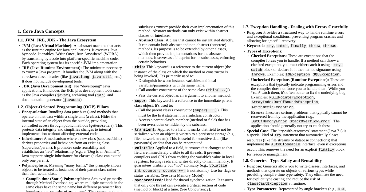
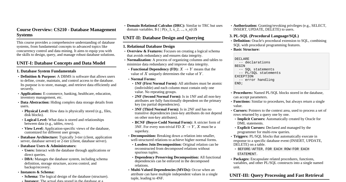
1. Introduction to DBMS A Database Management System (DBMS) is a software system that allows users to define, create, maintain, and control access to the database. It provides a structured way to store, retrieve, and manage large amounts of data efficiently. Database: A collection of interrelated data. DBMS: A software system that allows users to interact with the database. 1.1 DBMS vs. File System Traditionally, data was stored and managed using file systems. DBMS offers significant advantages over file systems: Data Redundancy and Inconsistency: File System: Data often duplicated across multiple files, leading to inconsistencies when updates are not applied everywhere. DBMS: Aims to reduce redundancy by centralizing data, enforcing integrity constraints. Difficulty in Accessing Data: File System: Requires writing new application programs for every new query or data access pattern. DBMS: Provides powerful query languages (like SQL) for flexible data retrieval without writing complex code. Data Isolation: File System: Data scattered in various files, different formats, making integration difficult. DBMS: Standardized data format and structure, promoting data integration. Integrity Problems: File System: Constraints (e.g., student age > 0) are embedded in application code, hard to change or enforce consistently. DBMS: Provides mechanisms (e.g., primary keys, foreign keys, CHECK constraints) to define and enforce data integrity rules centrally. Atomicity of Updates: File System: If a system fails during a multi-step update, data can be left in an inconsistent state (e.g., transfer money from A to B, money deducted from A but not added to B). DBMS: Ensures atomicity (all or nothing) through transactions and recovery mechanisms. Concurrent Access Issues: File System: Uncontrolled concurrent access can lead to inconsistent data (e.g., two users updating the same balance simultaneously). DBMS: Provides concurrency control mechanisms (e.g., locking) to manage simultaneous access and maintain data consistency. Security Problems: File System: Limited security controls, often at file level. DBMS: Offers fine-grained access control (e.g., specific users can only see certain columns or rows). Question: Explain how a DBMS overcomes the problem of 'data isolation' encountered in traditional file systems. 1.2 Data Models A data model is a collection of conceptual tools for describing data, data relationships, data semantics, and consistency constraints. ER Model (Entity-Relationship Model): High-level conceptual model. Used for database design (conceptual schema). Represents real-world entities and their relationships. Relational Model: The most widely used logical data model. Represents data as a collection of tables (relations). Each table has columns (attributes) and rows (tuples). Object-Based Data Models: Object-Oriented Data Model: Incorporates concepts of objects, classes, inheritance from OOP. Object-Relational Data Model: Extends the relational model with object-oriented features. Semi-structured Data Model: Allows data items of the same type to have different attributes. Examples: XML, JSON. 1.3 Schema and Instance Database Schema: The logical design or structure of the database. It describes the overall organization of data. It changes infrequently. Example: CUSTOMER (CustID, Name, Address, Phone) Database Instance: The actual content or data in the database at a particular point in time. It changes frequently. Example: (101, 'Alice', '123 Main St', '555-1234') Question: Differentiate between database schema and database instance with a real-world example. 1.4 Schema Architecture (Three-Schema Architecture) The ANSI/SPARC architecture defines three levels of abstraction: External Schema (View Level): Describes the part of the database that a particular user group is interested in. Hides irrelevant details and can customize the presentation of data. Multiple external schemas can exist for a single conceptual schema. Conceptual Schema (Logical Level): Describes the entire database structure for the community of users. Hides details of physical storage structures. Focuses on entities, attributes, relationships, and constraints. Internal Schema (Physical Level): Describes the physical storage structure of the database. Details how data is stored on disk (e.g., file organization, indexing, record placement). 1.5 Data Independence The ability to modify a schema at one level without affecting a schema at a higher level. Logical Data Independence: The ability to change the conceptual schema without having to change external schemas or application programs. Example: Adding a new attribute to a table in the conceptual schema doesn't require rewriting applications that don't use that attribute. Physical Data Independence: The ability to change the internal (physical) schema without having to change the conceptual schema. Example: Changing the file organization (e.g., from heap to B+-tree) or adding an index doesn't affect how users view the data logically. Question: A database administrator decides to add an index to a large table to improve query performance. Which type of data independence is primarily demonstrated here, and why? 1.6 Database Languages and Interfaces Data Definition Language (DDL): Used to define the database schema (create, modify, delete database objects). Commands: CREATE TABLE , ALTER TABLE , DROP TABLE , CREATE INDEX . CREATE TABLE Students ( StudentID INT PRIMARY KEY, Name VARCHAR(100), Major VARCHAR(50) ); Data Manipulation Language (DML): Used for accessing and manipulating data in the database. Commands: SELECT , INSERT , UPDATE , DELETE . INSERT INTO Students (StudentID, Name, Major) VALUES (1, 'Alice', 'CS'); SELECT * FROM Students WHERE Major = 'CS'; Data Control Language (DCL): Used to control access to data in the database (permissions). Commands: GRANT , REVOKE . Transaction Control Language (TCL): Used to manage transactions. Commands: COMMIT , ROLLBACK , SAVEPOINT . 1.7 Database Users and DBA Database Users: Naive Users: Interact with the system through pre-written application programs. Application Programmers: Develop application programs. Sophisticated Users: Interact with the system by writing queries directly (e.g., analysts). Specialized Users: Write specialized database applications that do not fit into the traditional data-processing framework (e.g., CAD systems, knowledge-based systems). Database Administrator (DBA): The person or team responsible for the overall control of the database system. Functions: Schema definition and modification. Storage structure and access method definition. Granting user authorization for data access. Monitoring database performance and responding to changes. Database backup and recovery. Data migration and upgrades. Question: Identify two key responsibilities of a Database Administrator (DBA) related to data security and availability. 2. Data Modeling using the Entity-Relationship (ER) Model The ER model is a high-level conceptual data model used to represent the overall logical structure of a database during the design phase. 2.1 ER Model Concepts Entity: A "thing" or "object" in the real world that is distinguishable from other objects. Examples: A specific student 'Alice', a course 'Database Systems'. Entity Set: A collection of similar entities (e.g., all students, all courses). Attribute: A property or characteristic describing an entity. Examples for Student entity: StudentID , Name , Age . Types of Attributes: Simple vs. Composite: Name (simple) vs. Address (composite: Street , City , Zip ). Single-valued vs. Multi-valued: Age (single) vs. Phone_Numbers (multi-valued). Derived: Can be computed from other attributes (e.g., Age from Date_of_Birth ). Key Attribute: Uniquely identifies an entity in an entity set (e.g., StudentID ). Relationship: An association among several entities. Examples: A student enrolls_in a course. Relationship Set: A collection of similar relationships. Degree of a Relationship Set: The number of entity sets participating in the relationship. Binary (degree 2): Student enrolls_in Course . Ternary (degree 3): Instructor teaches Course in Semester . Recursive Relationship: Relationship between entities of the same entity type (e.g., an Employee manages another Employee ). 2.2 Relationship Types and Constraints Cardinality Ratios (Mapping Cardinalities): Describe the number of entities to which another entity can be associated via a relationship set. One-to-One (1:1): An entity in A is associated with at most one entity in B, and vice-versa. (e.g., Employee manages Department ) One-to-Many (1:N): An entity in A is associated with multiple entities in B, but an entity in B is associated with at most one entity in A. (e.g., Department has Employees ) Many-to-One (N:1): An entity in A is associated with at most one entity in B, but an entity in B is associated with multiple entities in A. (e.g., Employees work_for Department ) Many-to-Many (M:N): An entity in A is associated with multiple entities in B, and an entity in B is associated with multiple entities in A. (e.g., Students enroll_in Courses ) Participation Constraints: Specify whether an entity must participate in a relationship. Total Participation: Every entity in the entity set must participate in at least one relationship instance. (e.g., Every Employee must work_for a Department ). Represented by a double line. Partial Participation: An entity in the entity set may or may not participate in the relationship. (e.g., A Manager may or may not manage a Project ). Represented by a single line. Weak Entity Sets: An entity set that does not have sufficient attributes to form a primary key. Its existence depends on another entity (identifying owner entity). The primary key of a weak entity set is formed by the primary key of its identifying owner entity plus its own partial key (discriminator). Represented by a double rectangle, and its identifying relationship by a double diamond. The partial key is underlined with a dashed line. Example: Dependent (of an Employee ) identified by Name within an Employee . Question: Design an ER diagram for a library system where books can be borrowed by members. A book can have multiple copies, and each copy can be borrowed by only one member at a time. A member can borrow multiple copies. Identify entity sets, attributes, relationship sets, and cardinality ratios. 2.3 Extended ER-Model Concepts (EER Model) Generalization: A bottom-up approach where common properties of two or more entity types are combined to form a higher-level entity type. Example: Car and Truck can be generalized into Vehicle . Specialization: A top-down approach where a higher-level entity type is divided into one or more lower-level entity types based on their specific characteristics. Example: Employee can be specialized into Secretary , Engineer , Technician . Constraints on Specialization: Disjointness: Disjoint: An entity can belong to at most one specialized entity set (e.g., an Employee cannot be both a Secretary and an Engineer simultaneously). Denoted by 'd'. Overlapping: An entity can belong to more than one specialized entity set (e.g., a Person can be both an Artist and an Employee ). Denoted by 'o'. Completeness: Total: Every entity in the higher-level entity set must belong to at least one of the lower-level entity sets (e.g., every Employee must be either a Secretary , Engineer , or Technician ). Denoted by a double line. Partial: An entity in the higher-level entity set may not belong to any of the lower-level entity sets. Denoted by a single line. Aggregation: Used to represent a relationship between a relationship and an entity. Treats a relationship set as an entity set for the purpose of participating in other relationships. Example: Project - Employee works_on relationship can be aggregated and then related to a Manager ( Manager supervises ( works_on relationship)). Question: Consider a university system. How would you use generalization and specialization to model different types of 'Person' (e.g., Student, Faculty, Staff) and their specific attributes? 2.4 Transforming ER Diagram into Tables (Relational Schema) The process of converting a conceptual ER model into a logical relational schema. Strong Entity Sets: Each strong entity set becomes a table (relation). Its attributes become columns. The key attribute becomes the primary key. STUDENT( StudentID , Name, Major) Weak Entity Sets: A weak entity set becomes a table. Its primary key is the combination of its partial key and the primary key of its identifying owner entity. DEPENDENT( EmpID , DependentName , Relationship) (where EmpID is FK to EMPLOYEE ) One-to-One (1:1) Relationship Sets: Option 1: Merge one of the entity sets into the other. Option 2: Create a separate table for the relationship, including primary keys from both participating entities (one of which is also a foreign key). Option 3: Add the primary key of one entity set as a foreign key to the other entity set's table. One-to-Many (1:N) Relationship Sets: The primary key of the "one" side entity is added as a foreign key to the "many" side entity's table. DEPARTMENT( DeptID , Name) , EMPLOYEE( EmpID , EmpName, DeptID) ( DeptID is FK to DEPARTMENT ) Many-to-Many (M:N) Relationship Sets: Create a new table for the relationship. This table includes the primary keys of all participating entity sets (which collectively form its primary key and are foreign keys to their respective tables), plus any attributes of the relationship itself. STUDENT( StudentID , Name) , COURSE( CourseID , Title) ENROLLS( StudentID , CourseID , Grade) ( StudentID FK to STUDENT , CourseID FK to COURSE ) Multi-valued Attributes: Create a new table for the multi-valued attribute. This table includes the primary key of the entity set and the multi-valued attribute itself. EMPLOYEE( EmpID , Name) , EMP_PHONE( EmpID , PhoneNumber ) Composite Attributes: Each component of the composite attribute becomes a separate column. Address (Street, City, Zip) $\to$ Street , City , Zip columns. Generalization/Specialization: Option 1 (Separate tables for all): Create a table for the higher-level entity and separate tables for each lower-level entity. Lower-level tables include the primary key of the higher-level table (as both primary key and foreign key). Option 2 (Separate tables for lower-level only): Create tables only for the lower-level entities. Each table includes all attributes of the higher-level entity plus its own specific attributes. (Applicable for total, disjoint specialization). Option 3 (Single table): Create one table for the higher-level entity, including all attributes of all lower-level entities, plus a type attribute to indicate the specialization. (Can lead to many NULLs). Question: Given an ER diagram with a many-to-many relationship "Works_On" between "Employee" and "Project" entities, with an attribute "Hours" on the relationship. Describe how you would transform this into relational tables, specifying primary and foreign keys. 3. Relational Data Models 3.1 Domains, Tuples, Attributes, Relations Domain: A set of atomic values. Each attribute in a relation must draw its values from a specific domain. Example: The domain of Age could be integers from 0 to 150. Attribute: A named column of a relation, representing a specific property. Tuple: A row in a relation, representing a single record or instance of an entity. Relation: A table composed of a schema and an instance. Relation Schema: $R = (A_1, A_2, ..., A_n)$, where $R$ is the relation name and $A_i$ are the attributes. Relation Instance: A set of tuples $r = \{t_1, t_2, ..., t_m\}$, where each $t_j$ is a tuple. 3.2 Characteristics of Relations Order of Tuples: The order of tuples (rows) in a relation is theoretically insignificant. Order of Attributes: The order of attributes (columns) is theoretically insignificant, but practically meaningful for readability. Atomic Values: Each cell in a relation contains a single, indivisible value. Multi-valued attributes are not directly supported. Unique Tuples: A relation cannot have duplicate tuples (rows). 3.3 Keys Superkey: A set of one or more attributes that, taken collectively, uniquely identifies a tuple within a relation. If $K$ is a superkey, then any superset of $K$ is also a superkey. Candidate Key: A minimal superkey; no proper subset of its attributes can uniquely identify tuples. A relation can have multiple candidate keys. Primary Key: One of the candidate keys chosen by the database designer to uniquely identify tuples in a relation. It is usually underlined in schema notation. Primary key attributes cannot have NULL values. Alternate Key: A candidate key that is not chosen as the primary key. Foreign Key: A set of attributes in a relation that refers to the primary key of another relation (or the same relation). It establishes a link between tables and enforces referential integrity. The domain of the foreign key attributes must be compatible with the domain of the primary key attributes it references. Foreign key values can be NULL if the foreign key is not part of the primary key of its own table, unless explicitly constrained otherwise. Question: In a STUDENT table with attributes ( StudentID , Name , Email , SSN ), assume StudentID , Email , and SSN are all unique. Identify all candidate keys, the primary key (if StudentID is chosen), and any alternate keys. 3.4 Integrity Constraints Rules that ensure the quality and consistency of data in a database. Domain Constraints: Each attribute value must be from its specified domain. Entity Integrity Constraint: The primary key of a relation cannot contain NULL values. This ensures that every tuple can be uniquely identified. Referential Integrity Constraint: If a foreign key in relation $R_1$ refers to the primary key of relation $R_2$, then every value of the foreign key in $R_1$ must either be equal to a value of the primary key in $R_2$ or be NULL. Actions on Delete/Update of Referenced Primary Key: Restrict: Prevent deletion/update if there are referencing foreign key values. Cascade: Delete/update referencing foreign key values as well. Set Null: Set referencing foreign key values to NULL. Set Default: Set referencing foreign key values to a default value. Check Constraints: User-defined conditions that a column's values must satisfy. Example: CHECK (Salary > 0) Question: Explain why NULL values are generally not allowed in a primary key, relating your answer to the purpose of a primary key. 3.5 Relational Algebra A procedural query language that takes relations as input and produces relations as output. It forms the theoretical basis for SQL. Unary Operations (operate on a single relation): Selection ($\sigma$): Selects a subset of tuples from a relation that satisfy a selection condition $P$. Notation: $\sigma_P(R)$ Example: Find all students majoring in 'CS'. $\sigma_{\text{Major = 'CS'}}(\text{STUDENT})$ Projection ($\pi$): Selects a subset of attributes (columns) from a relation. Eliminates duplicate tuples by default. Notation: $\pi_{A_1, A_2, ..., A_k}(R)$ Example: Get the names of all students. $\pi_{\text{Name}}(\text{STUDENT})$ Rename ($\rho$): Renames a relation or its attributes. Notation: $\rho_{S(B_1, ..., B_n)}(R)$ (renames relation $R$ to $S$ and its attributes to $B_1, ..., B_n$). Notation: $\rho_S(R)$ (renames relation $R$ to $S$). Binary Operations (operate on two relations): Union ($\cup$): $R \cup S$ includes all tuples that are in $R$, or in $S$, or in both. Requires relations to be union-compatible (same number of attributes, corresponding attributes have compatible domains). Set Difference ($-$): $R - S$ includes all tuples that are in $R$ but not in $S$. Requires union-compatibility. Cartesian Product ($\times$): $R \times S$ combines every tuple from $R$ with every tuple from $S$. If $R$ has $n$ tuples and $S$ has $m$ tuples, $R \times S$ has $n \times m$ tuples. Natural Join ($\bowtie$): $R \bowtie S$ combines tuples from $R$ and $S$ that have identical values on their common attributes. It automatically performs an equality test on all common attributes and then projects out the duplicate common attributes. Example: Combine STUDENT and ENROLLS relations on StudentID . $\text{STUDENT} \bowtie \text{ENROLLS}$ Theta Join ($\bowtie_\theta$): $R \bowtie_\theta S = \sigma_\theta (R \times S)$. Combines tuples from $R$ and $S$ that satisfy a join condition $\theta$. Equijoin: A theta join where the join condition $\theta$ consists only of equality comparisons. Derived Operations: Intersection ($\cap$): $R \cap S = R - (R - S)$. Division ($\div$): Used for "for all" queries. $R \div S$ contains tuples from $R$ that match all tuples in $S$ on certain attributes. Question: Write a relational algebra expression to find the names of students who have enrolled in 'Database Systems' course. Assume relations STUDENT( StudentID , Name, Major) , COURSE( CourseID , Title) , and ENROLLS( StudentID , CourseID ) . 3.6 Relational Calculus A non-procedural query language where users specify what data they want, not how to retrieve it. Tuple Relational Calculus (TRC): Form: $\{t \mid P(t)\}$, where $t$ is a tuple variable and $P(t)$ is a predicate expression involving $t$. Uses quantifiers: $\exists$ (there exists), $\forall$ (for all). Example: Find all student IDs and names for students in the 'CS' department. $\{t \mid t \in \text{STUDENT} \land t[\text{Major}] = \text{'CS'}\}$ Example with projection: $\{t \mid \exists s \in \text{STUDENT}(t[\text{Name}] = s[\text{Name}] \land s[\text{Major}] = \text{'CS'})\}$ Domain Relational Calculus (DRC): Form: $\{\langle x_1, x_2, ..., x_n \rangle \mid P(x_1, x_2, ..., x_n)\}$, where $x_i$ are domain variables. Example: Find all student IDs and names for students in the 'CS' department. $\{\langle \text{sid, sname} \rangle \mid \exists \text{major} (\langle \text{sid, sname, major} \rangle \in \text{STUDENT} \land \text{major} = \text{'CS'})\}$ Safety: A relational calculus expression is "safe" if it is guaranteed to produce a finite result relation. Unsafe expressions can lead to infinite results (e.g., "all tuples not in R"). Question: Write a Tuple Relational Calculus expression to find the names of students who have not enrolled in any course. 4. SQL (Structured Query Language) The most widely used declarative language for relational databases. 4.1 Basic SQL Query Structure SELECT [DISTINCT] attribute_list FROM table_list [WHERE condition] [GROUP BY grouping_attributes] [HAVING group_condition] [ORDER BY sorting_attributes [ASC|DESC]]; SELECT : Specifies the attributes to be retrieved. DISTINCT removes duplicate rows. * selects all columns. Example: SELECT DISTINCT Major FROM Students; FROM : Specifies the tables involved in the query. WHERE : Filters rows based on a condition. Operators: =, , =, <>, LIKE, IN, BETWEEN, IS NULL, AND, OR, NOT . Example: SELECT * FROM Students WHERE Age > 20 AND Major = 'CS'; LIKE : For pattern matching ( % for any sequence of characters, _ for any single character). Example: SELECT Name FROM Students WHERE Name LIKE 'A%'; 4.2 Creating Table and Views Creating Tables (DDL): CREATE TABLE Course ( CourseID VARCHAR(10) PRIMARY KEY, Title VARCHAR(100) NOT NULL, Credits INT CHECK (Credits > 0), DeptName VARCHAR(50), FOREIGN KEY (DeptName) REFERENCES Department(DeptName) ON DELETE CASCADE ); Constraints: PRIMARY KEY , FOREIGN KEY , NOT NULL , UNIQUE , CHECK . ON DELETE CASCADE : If a referenced row is deleted, delete referencing rows. ON DELETE SET NULL : If a referenced row is deleted, set referencing foreign key to NULL. Creating Views: A virtual table based on the result-set of an SQL statement. Views do not store data themselves; they are derived from base tables. CREATE VIEW CS_Students AS SELECT StudentID, Name FROM Students WHERE Major = 'CS'; Views can simplify queries, enhance security (hide columns/rows), and provide logical data independence. Updates through views are complex and restricted. 4.3 SQL as DML, DDL, DCL DDL (Data Definition Language): CREATE TABLE, ALTER TABLE, DROP TABLE, CREATE VIEW, DROP VIEW, CREATE INDEX, DROP INDEX . DML (Data Manipulation Language): INSERT INTO table_name (columns) VALUES (values); UPDATE table_name SET column1 = value1 WHERE condition; DELETE FROM table_name WHERE condition; DCL (Data Control Language): GRANT privileges ON object TO user; REVOKE privileges ON object FROM user; TCL (Transaction Control Language): COMMIT, ROLLBACK, SAVEPOINT . 4.4 SQL Algebraic Operations (Set Operations) UNION: Combines the result sets of two or more SELECT statements. Removes duplicate rows by default. SELECT Name FROM Faculty UNION SELECT Name FROM Staff; UNION ALL: Combines results, retaining duplicate rows. INTERSECT: Returns only the rows that are common to both result sets. SELECT Name FROM Students INTERSECT SELECT Name FROM Employees; EXCEPT (or MINUS in Oracle): Returns rows from the first query that are not present in the second query. SELECT Name FROM Students EXCEPT SELECT Name FROM Graduates; 4.5 Joins Combine rows from two or more tables based on a related column between them. INNER JOIN (or simply JOIN): Returns rows when there is at least one match in both tables. SELECT S.Name, E.CourseID FROM Students S INNER JOIN Enrolls E ON S.StudentID = E.StudentID; LEFT (OUTER) JOIN: Returns all rows from the left table, and the matching rows from the right table. If no match, NULLs are returned for right table columns. SELECT S.Name, E.CourseID FROM Students S LEFT JOIN Enrolls E ON S.StudentID = E.StudentID; -- Shows all students, even those not enrolled in any course RIGHT (OUTER) JOIN: Returns all rows from the right table, and the matching rows from the left table. FULL (OUTER) JOIN: Returns all rows when there is a match in one of the tables. CROSS JOIN (Cartesian Product): Returns the Cartesian product of the two tables. NATURAL JOIN: Joins tables automatically on all columns with matching names and data types. SELF JOIN: A table joined with itself, useful for comparing rows within the same table. Requires aliasing. SELECT A.Name AS Student1, B.Name AS Student2 FROM Students A, Students B WHERE A.Major = B.Major AND A.StudentID Question: Explain the difference between an INNER JOIN and a LEFT JOIN . Provide a scenario where a LEFT JOIN would be more appropriate than an INNER JOIN . 4.6 Sub-Queries (Nested Queries) A query embedded inside another SQL query. In WHERE clause: SELECT Name FROM Students WHERE StudentID IN (SELECT StudentID FROM Enrolls WHERE CourseID = 'CS101'); With EXISTS / NOT EXISTS : Tests for the existence of rows returned by the subquery. SELECT Name FROM Students S WHERE EXISTS (SELECT * FROM Enrolls E WHERE E.StudentID = S.StudentID AND E.CourseID = 'CS101'); With ALL / ANY (or SOME ): Compares a value with every value ( ALL ) or at least one value ( ANY / SOME ) returned by the subquery. SELECT Name FROM Students WHERE Age > ALL (SELECT Age FROM Faculty); -- Older than all faculty members Scalar Subquery: Returns a single value, can be used anywhere a single value is expected. SELECT Name, (SELECT AVG(Credits) FROM Course) AS AvgCourseCredits FROM Students; FROM clause (Derived Tables): SELECT T.DeptName, T.AvgSalary FROM (SELECT DeptName, AVG(Salary) AS AvgSalary FROM Instructor GROUP BY DeptName) AS T WHERE T.AvgSalary > 60000; WITH clause (Common Table Expressions - CTEs): Provides a way to define a temporary named result set that you can reference within a single SELECT , INSERT , UPDATE , or DELETE statement. WITH DeptAvgSalary (DeptName, AvgSal) AS ( SELECT DeptName, AVG(Salary) FROM Instructor GROUP BY DeptName ) SELECT D.DeptName, D.AvgSal FROM DeptAvgSalary D WHERE D.AvgSal > 60000; 4.7 Aggregate Operations Functions that operate on a set of rows and return a single summary value. Functions: COUNT(), SUM(), AVG(), MIN(), MAX() . GROUP BY clause: Groups rows that have the same values in specified columns into summary rows, allowing aggregate functions to operate on each group. SELECT DeptName, AVG(Salary) AS AverageSalary FROM Instructor GROUP BY DeptName; HAVING clause: Filters groups based on conditions applied to aggregate functions. It is applied after GROUP BY . SELECT DeptName, AVG(Salary) FROM Instructor GROUP BY DeptName HAVING AVG(Salary) > 70000; Difference between WHERE and HAVING : WHERE filters individual rows before grouping, HAVING filters groups after grouping. Question: Write an SQL query to find the department names that have more than 5 instructors, along with the count of instructors in those departments. 4.8 Cursors A database object that enables traversal over the rows of a result set, one row at a time. Used in procedural contexts (e.g., stored procedures, application programs) to process data row by row. Steps: DECLARE: Define the cursor based on a SELECT statement. OPEN: Execute the SELECT statement and populate the result set. FETCH: Retrieve one row at a time from the result set. CLOSE: Release the resources held by the cursor. DEALLOCATE: Remove the cursor definition. Types: Read-only, scrollable, updateable. 4.9 Dynamic SQL SQL statements constructed and executed at runtime, rather than being hardcoded. This allows for more flexible and adaptable applications. Uses: Building ad-hoc queries, creating generic reporting tools, performing DDL operations from within application code. Risks: SQL Injection vulnerabilities if input is not properly sanitized. 4.10 Integrity Constraints in SQL SQL provides robust mechanisms to define and enforce integrity constraints: PRIMARY KEY : Uniquely identifies each row, implicitly NOT NULL and UNIQUE . FOREIGN KEY : Enforces referential integrity. NOT NULL : Ensures a column cannot have NULL values. UNIQUE : Ensures all values in a column (or set of columns) are distinct. Can contain NULLs. CHECK : Defines a condition that all values in a column must satisfy. CREATE TABLE Product ( ProductID INT PRIMARY KEY, Price DECIMAL(10, 2) CHECK (Price >= 0), Category VARCHAR(50) ); 4.11 Triggers A special type of stored procedure that automatically executes (fires) when a specific event occurs in the database. Events: INSERT , UPDATE , DELETE . Timing: BEFORE or AFTER the event. Granularity: Row-level trigger: Fires once for each row affected by the event. (e.g., FOR EACH ROW ) Statement-level trigger: Fires once per statement, regardless of the number of rows affected. Uses: Enforcing complex business rules, auditing changes, maintaining derived data, implementing complex referential integrity actions. CREATE TRIGGER trg_AfterInsertStudent AFTER INSERT ON Students FOR EACH ROW BEGIN -- Log the new student insertion INSERT INTO AuditLog (Action, Timestamp) VALUES ('New student ' || NEW.Name || ' added', NOW()); END; Question: Describe a scenario where a database trigger would be a suitable solution to maintain data consistency or implement a business rule. 5. Database Design: Normalization A systematic approach to organizing the columns and tables of a relational database to minimize data redundancy and improve data integrity. 5.1 Functional Dependency (FD) An integrity constraint between two sets of attributes in a relation. $A \to B$ means that if two tuples have the same value for attributes in $A$, then they must also have the same value for attributes in $B$. ($A$ uniquely determines $B$). Example: StudentID $\to$ StudentName (StudentID determines StudentName). Trivial FD: $A \to B$ where $B \subseteq A$. (e.g., {StudentID, Name} $\to$ Name ) 5.2 Normal Forms A series of guidelines for designing robust databases. Each normal form addresses specific types of data redundancy and anomaly problems. 1st Normal Form (1NF): A relation is in 1NF if all attribute values are atomic (indivisible) and each column contains values from a single domain. No multi-valued attributes or nested relations. 2nd Normal Form (2NF): A relation is in 2NF if it is in 1NF and every non-key attribute is fully functionally dependent on the primary key. No partial dependencies (where a non-key attribute depends on only part of a composite primary key). Problem: If {StudentID, CourseID} is PK, and CourseID $\to$ CourseTitle , then CourseTitle is partially dependent. 3rd Normal Form (3NF): A relation is in 3NF if it is in 2NF and there are no transitive dependencies. A transitive dependency exists when a non-key attribute is functionally dependent on another non-key attribute. (i.e., $A \to B$ and $B \to C$, then $A \to C$ is a transitive dependency). Problem: If StudentID $\to$ DeptName and DeptName $\to$ DeptHead , then StudentID $\to$ DeptHead is transitive. Boyce-Codd Normal Form (BCNF): A relation is in BCNF if for every non-trivial functional dependency $A \to B$, $A$ is a superkey. A stricter form of 3NF. It handles cases where 3NF fails (e.g., when a non-key attribute determines part of a candidate key). Every BCNF relation is in 3NF, but not vice-versa. 4th Normal Form (4NF): A relation is in 4NF if it is in BCNF and contains no multi-valued dependencies (MVDs). Multi-valued Dependency (MVD): $A \twoheadrightarrow B$ means that for each $A$ value, there is a set of $B$ values, and this set is independent of other attributes. Example: Student $\twoheadrightarrow$ Hobby and Student $\twoheadrightarrow$ Language . 5th Normal Form (5NF) / Project-Join Normal Form (PJNF): A relation is in 5NF if it is in 4NF and contains no join dependencies (JDs). A JD exists if a relation can be reconstructed by joining smaller relations, but cannot be decomposed into smaller relations without loss of information. Question: Consider a table EMP_PROJ( EmpID , ProjID , EmpName, ProjName, ProjLocation) . Assume EmpID $\to$ EmpName , ProjID $\to$ ProjName, ProjLocation . Is this table in 2NF? If not, explain why and decompose it into 2NF. 5.3 Decomposition The process of breaking down a relation into smaller, "well-behaved" relations (i.e., in higher normal forms). Lossless Join Decomposition: A decomposition $R$ into $R_1, R_2, ..., R_n$ is lossless if the natural join of all $R_i$ produces exactly the original relation $R$. Test for binary decomposition $R$ into $R_1, R_2$: $(R_1 \cap R_2) \to (R_1 - R_2)$ or $(R_1 \cap R_2) \to (R_2 - R_1)$ must hold. Dependency Preservation: A decomposition is dependency-preserving if all original functional dependencies can be enforced by enforcing FDs in the decomposed relations. Normalization aims for both lossless join and dependency preservation, but sometimes a trade-off is necessary (especially between BCNF and 3NF). 5.4 Armstrong's Axioms A set of inference rules for functional dependencies. Used to find all FDs implied by a given set of FDs. Reflexivity: If $B \subseteq A$, then $A \to B$. (Trivial dependencies) Augmentation: If $A \to B$, then $AC \to BC$ (where $C$ is any set of attributes). Transitivity: If $A \to B$ and $B \to C$, then $A \to C$. Derived Rules: Union: If $A \to B$ and $A \to C$, then $A \to BC$. Decomposition: If $A \to BC$, then $A \to B$ and $A \to C$. Pseudotransitivity: If $A \to B$ and $CB \to D$, then $AC \to D$. Question: Given FDs $A \to B$ and $B \to C$, use Armstrong's axioms to prove that $A \to C$. 5.5 Canonical Cover A minimal set of functional dependencies that is equivalent to a given set of FDs $F$. It satisfies three properties: Every FD in $F_c$ (canonical cover) has a single attribute on the right-hand side. No attribute on the left-hand side of an FD in $F_c$ is redundant. No FD in $F_c$ is redundant (i.e., cannot be inferred from other FDs in $F_c$). Algorithm to find canonical cover: Convert all FDs to have a single attribute on the RHS. For each FD $X \to A$: For each attribute $B \in X$: check if $(X - \{B\}) \to A$ can be derived. If yes, remove $B$ from $X$. For each FD $X \to A$: check if $X \to A$ can be derived from other FDs in the set. If yes, remove $X \to A$. 5.6 Problems with Null Values and Dangling Tuples Null Values: Can cause ambiguity in join operations (e.g., WHERE A=B might not match NULL=NULL ). Can complicate aggregate functions (e.g., AVG() ignores NULLs). Can make integrity constraint enforcement difficult. Dangling Tuples: Occur when a foreign key references a primary key that no longer exists (violation of referential integrity). Can lead to inconsistent data and incorrect query results. 5.7 Multivalued Dependencies (MVDs) $A \twoheadrightarrow B$ exists in relation $R$ if, for any two tuples in $R$ that agree on $A$, their $B$ values can be swapped, and the resulting tuples are also in $R$. This means $B$ is multi-valued and independent of other attributes in $R - A - B$. Example: Course $\twoheadrightarrow$ Textbook and Course $\twoheadrightarrow$ Instructor means that for a given course, the set of textbooks is independent of the set of instructors. MVDs are handled by 4NF. Question: A table STUDENT_SKILL_CLUB( StudentID , Skill, Club) has the following data for student S1: (S1, Python, Chess), (S1, Python, Debate), (S1, Java, Chess), (S1, Java, Debate). Identify if there's an MVD present and explain why. 6. Transaction Processing Concepts A transaction is a unit of program execution that accesses and possibly updates various data items. 6.1 Transaction Properties (ACID) Atomicity: The "all or nothing" property. Either all operations within a transaction complete successfully, or none of them do. If a transaction fails, all its partial changes are undone (rolled back). Consistency: A transaction must transform the database from one valid and consistent state to another. It preserves all defined integrity constraints. Isolation: Concurrent execution of transactions should produce the same result as if they were executed serially (one after another). Each transaction is unaware of other concurrent transactions. Durability: Once a transaction is committed, its changes are permanently stored in the database and survive any subsequent system failures (e.g., power outage). Question: A bank transaction involves transferring money from Account A to Account B. Explain how the ACID properties ensure this transaction is processed reliably. 6.2 Transaction States Active: The initial state; the transaction is executing its operations. Partially Committed: After the last statement of the transaction has been executed. Changes are in main memory but not yet on stable storage. Committed: After all changes have been successfully and permanently stored on stable storage. The transaction has completed successfully. Failed: The transaction cannot proceed normally (e.g., integrity constraint violation, system error). Aborted: After the transaction has been rolled back and the database restored to its state before the transaction began. The transaction may then be restarted or terminated. 6.3 Schedules A sequence of operations (read, write, commit, abort) from a set of concurrent transactions. Serial Schedule: Transactions execute one after another, without any interleaving of operations. Always correct (consistent and isolated). Concurrent Schedule: Operations from multiple transactions are interleaved. Can improve throughput but introduces potential consistency issues. 6.4 Serializability of Schedules A concurrent schedule is serializable if it is equivalent to some serial schedule. This ensures that the database remains consistent even with concurrency. Conflict Serializability: Two operations conflict if they belong to different transactions, access the same data item, and at least one of them is a write operation. A schedule is conflict serializable if it can be transformed into a serial schedule by swapping non-conflicting operations. Precedence Graph (or Serialization Graph): A directed graph where nodes are transactions and an edge $T_i \to T_j$ exists if $T_i$ conflicts with $T_j$ and $T_i$'s conflicting operation occurs before $T_j$'s. If the graph is acyclic, the schedule is conflict serializable. View Serializability: A more general notion than conflict serializability. Two schedules $S$ and $S'$ are view equivalent if: For each data item $Q$, if $T_i$ reads $Q$ in $S$, then $T_i$ must read the initial value of $Q$ in $S'$, or $T_j$ must write $Q$ before $T_i$ reads $Q$ in both $S$ and $S'$. For each write $Q$ by $T_i$ in $S$, if $T_i$ is the final writer of $Q$ in $S$, then $T_i$ must also be the final writer of $Q$ in $S'$. A schedule is view serializable if it is view equivalent to some serial schedule. Difficult to test algorithmically (NP-complete). Question: Given two transactions $T_1: R(A), W(A), R(B), W(B)$ and $T_2: R(A), W(A), R(B), W(B)$. Consider the schedule $S: R_1(A), R_2(A), W_1(A), W_2(A), R_1(B), R_2(B), W_1(B), W_2(B)$. Is this schedule conflict serializable? Explain using a precedence graph. 6.5 Recoverability Ensures that if a transaction fails, its effects can be undone without affecting other committed transactions. Recoverable Schedule: If a transaction $T_j$ reads a data item written by $T_i$, then $T_i$ must commit before $T_j$ commits. This prevents $T_j$ from committing based on a value that might later be undone if $T_i$ aborts. Cascading Rollbacks: If $T_j$ reads data written by $T_i$, and $T_i$ aborts, then $T_j$ must also abort. This propagates rollbacks. Cascadeless Schedule: A schedule where a transaction is only allowed to read data items written by other transactions that have already committed. This prevents cascading rollbacks. Strict Schedule: A schedule where a transaction can neither read nor write an item $X$ until the last transaction that wrote $X$ has committed or aborted. This is the strictest form and simplifies recovery. 6.6 Recovery from Transaction Failures The process of restoring the database to a consistent state after a failure. Log-Based Recovery: A log (or journal) is maintained on stable storage, recording all updates to the database. Each log record contains: transaction ID, data item ID, old value, new value. <start T_i> : Transaction $T_i$ has started. <T_i, X, V_1, V_2> : Transaction $T_i$ changed data item $X$ from $V_1$ to $V_2$. <commit T_i> : Transaction $T_i$ has committed. <abort T_i> : Transaction $T_i$ has aborted. Undo: Restore data item $X$ to $V_1$ (old value). Redo: Set data item $X$ to $V_2$ (new value). Write-Ahead Logging (WAL) Rule: Before a data item's new value is written to disk, the log record for that update must be written to disk. Before a transaction commits, all its log records must be written to disk. Checkpoints: A mechanism to reduce the amount of work needed during recovery. Periodically, the system: Forces all log records currently in main memory to stable storage. Forces all modified buffer blocks to stable storage. Writes a <checkpoint L> record to the log, where $L$ is the list of active transactions. Recovery only needs to consider transactions active at the last checkpoint and those that started after it. Question: Explain the purpose of a 'log' in database recovery and describe the two main types of operations (undo/redo) performed using it. 7. Concurrency Control Techniques Mechanisms to ensure that concurrent transactions execute correctly and maintain database consistency. 7.1 Concept of Locks A lock is a mechanism to control concurrent access to a data item. A transaction must acquire a lock on a data item before it can access it. Shared Lock (S-lock): Allows reading the data item. Multiple transactions can hold S-locks on the same item concurrently. Exclusive Lock (X-lock): Allows both reading and writing the data item. Only one transaction can hold an X-lock on an item at any time. Lock Compatibility Matrix: S X S Yes No X No No 7.2 Concurrency Control Protocols - Two-Phase Locking (2PL) A protocol that ensures conflict serializability by regulating when transactions can acquire and release locks. Phases: Growing Phase: A transaction can acquire locks but cannot release any locks. Shrinking Phase: A transaction can release locks but cannot acquire any new locks. Once a transaction releases a lock, it enters the shrinking phase and cannot acquire any more locks. Guarantees: Conflict serializability. Drawbacks: Can lead to deadlocks. Does not guarantee freedom from cascading rollbacks (unless strict). Strict 2PL: Holds all exclusive locks until the transaction commits or aborts. Guarantees cascadelessness and strictness. Widely used. Rigorous 2PL: Holds all locks (shared and exclusive) until the transaction commits or aborts. Even stricter. Question: Explain how the Two-Phase Locking (2PL) protocol prevents non-serializable schedules. What is a common drawback of using 2PL? 7.3 Deadlock Handling A situation where two or more transactions are waiting indefinitely for each other to release locks. Deadlock Prevention: Design protocols to ensure deadlocks never occur. Wait-Die Scheme: Older transactions wait for younger ones; younger ones die (rollback) if they request a resource held by an older one. Wound-Wait Scheme: Older transactions wound (force rollback) younger ones holding needed resources; younger ones wait for older ones. Requires timestamps for transactions. Deadlock Detection: Allow deadlocks to occur, then detect and resolve them. Wait-for Graph: A directed graph where an edge $T_i \to T_j$ means $T_i$ is waiting for $T_j$ to release a lock. A cycle in the graph indicates a deadlock. Resolution: Choose a victim transaction (e.g., one with minimal cost, fewest locks). Rollback the victim transaction. 7.4 Time-Stamping Protocols Assigns a unique timestamp to each transaction ($TS(T_i)$). Concurrency control is based on these timestamps. Older transactions (smaller timestamps) have priority. For each data item $X$, maintain: $W-timestamp(X)$: Largest timestamp of any transaction that successfully wrote $X$. $R-timestamp(X)$: Largest timestamp of any transaction that successfully read $X$. Read operation by $T_i$ on $X$: If $TS(T_i) Else: Read $X$. Set $R-timestamp(X) = max(R-timestamp(X), TS(T_i))$. Write operation by $T_i$ on $X$: If $TS(T_i) If $TS(T_i) Else: Write $X$. Set $W-timestamp(X) = TS(T_i)$. Guarantees: Serializability (equivalent to a serial schedule ordered by timestamps). Drawbacks: Can lead to many rollbacks. Does not guarantee cascadelessness. Thomas' Write Rule: If $TS(T_i) Question: How does a timestamp-based concurrency control protocol handle a read request from a transaction $T_i$ if the timestamp of $T_i$ is older than the write-timestamp of the data item it wants to read? 7.5 Validation-Based Protocol (Optimistic Concurrency Control) Assumes conflicts are rare. Transactions execute without acquiring locks, and validation occurs only at commit time. Phases for each transaction $T_i$: Read Phase: $T_i$ reads data items. All writes are to local copies. Validation Phase: $T_i$ checks if its local changes would violate serializability. Determines if $T_i$ can commit. Write Phase: If validation succeeds, $T_i$'s local changes are written to the database. Validation Test: For a transaction $T_i$ to commit, for all $T_j$ that committed while $T_i$ was running, one of the following must hold: $T_j$ finished its write phase before $T_i$ started its read phase. $T_j$ finished its read phase before $T_i$ started its read phase, and $T_i$'s read set and $T_j$'s write set do not overlap. $T_i$'s read set and $T_j$'s write set do not overlap, and $T_j$'s write set and $T_i$'s write set do not overlap. Advantages: Maximizes concurrency (no locking overhead during execution). Good for read-heavy workloads. Disadvantage: High rollback rate if conflicts are frequent (wastes work). 7.6 Multiple Granularity Allows data items to be locked at different levels of granularity (e.g., database, file, block, record). This can increase concurrency. Hierarchy of Locking: Database $\to$ Area $\to$ File $\to$ Record. Intention Locks: Used to indicate intent to lock at a finer granularity. Intention Shared (IS): Intent to set S-locks at a lower level. Intention Exclusive (IX): Intent to set X-locks at a lower level. Shared and Intention Exclusive (SIX): Holds an S-lock on the higher-level item, and an IX-lock on a lower-level item. A transaction must acquire an appropriate intention lock on a higher-level item before it can acquire a regular lock on a lower-level item. 7.7 Multiversion Schemes Maintains multiple versions of a data item. When a transaction needs to read a data item, it reads an appropriate old version, allowing it to proceed without waiting for writers. Multiversion Timestamp Ordering: Each write creates a new version with the writer's timestamp. Readers can always access the latest version with a timestamp less than or equal to their own. Multiversion Two-Phase Locking: Read-only transactions can read the latest committed version without locking. Update transactions still use 2PL for the latest version. Advantages: Increased concurrency, especially for read-only transactions. Disadvantages: Increased storage overhead for multiple versions. 7.8 Recovery with Concurrent Transactions The recovery manager needs to handle the interaction of multiple transactions during recovery. ARIES (Algorithm for Recovery and Isolation Exploiting Semantics): A widely used recovery algorithm that handles concurrent transactions efficiently. Uses a "redo-undo" approach. Maintains Log Sequence Numbers (LSNs) for log records and PageLSNs for database pages. Fuzzy checkpointing allows transactions to continue during checkpointing. Three passes during recovery: Analysis Pass: Reads log from last checkpoint to determine dirty pages and active transactions. Redo Pass: Reapplies all updates (committed or uncommitted) to bring database to state at time of crash (repeats history). Undo Pass: Rolls back uncommitted transactions identified in the analysis pass. Question: Describe the main idea behind multiversion concurrency control schemes and how they aim to improve concurrency compared to traditional locking. 8. File Structures How data is organized and stored on secondary storage (disks). 8.1 File Organization Heap File Organization: Records are placed in any free space available in the file. No specific order. Good for small files or when records are frequently inserted/deleted. Full table scans are efficient, but direct access by key is slow (requires scanning). Sequential File Organization: Records are stored in a physical sequence based on the value of a search key. Efficient for sequential access (e.g., reports, batch processing). Updates (insertions/deletions) can be expensive as they may require reorganizing the file. Clustered File Organization: Records are grouped together based on a common attribute value across multiple tables. Useful for queries involving joins frequently (e.g., Department and its Employees are stored physically close). Only one clustered index can exist per table. Hashing File Organization: A hash function converts a search key into an address (bucket) where the record is stored. Provides very fast direct access if the hash function distributes keys evenly. Static Hashing: Fixed number of buckets. Collisions handled by overflow chains. Dynamic Hashing (Extendable Hashing): The number of buckets grows or shrinks dynamically as data changes, reducing overflow. Question: When would a 'heap file organization' be preferred over a 'sequential file organization' for storing data, and what are its main disadvantages? 8.2 Indexing A data structure that improves the speed of data retrieval operations on a database table at the cost of additional writes and storage space to maintain the index data structure. Primary Index (Clustering Index): Defined on the primary key of a file. The data records are physically sorted and stored in the order of the primary index key. There can be only one primary index per file. Secondary Index (Non-clustering Index): Defined on any non-primary key attribute(s). The data records are not physically ordered according to the secondary index key. Contains pointers to the actual data records. Multiple secondary indexes can exist on a file. Dense Index: An index record appears for every search-key value in the data file. Sparse Index: An index record appears only for some (e.g., the first) search-key values in the data file. Only applicable for sequentially ordered files. 8.3 Multilevel Indexing with B-Tree, B+ Tree These are tree-based data structures designed for disk-based storage, optimized for minimizing disk I/O. B-Tree: A self-balancing search tree. Each node can have multiple children (typically 3-200). Nodes can store both keys and data pointers (or full data records). Internal nodes can contain data pointers. All leaf nodes are at the same depth. B+-Tree: The most common indexing structure in databases. All data pointers (or actual data records in clustering B+-trees) are stored only at the leaf nodes. Internal nodes only store key values and pointers to child nodes (acting as an index to the leaf nodes). Leaf nodes are linked together sequentially, allowing for efficient range queries. All leaf nodes are at the same depth. Advantages over B-Tree: More efficient range queries due to linked leaf nodes. More keys can fit in internal nodes, leading to a shallower tree and fewer disk I/Os for large datasets. Operations: Search: Traverse from root to leaf. Insertion: Find leaf, insert. If leaf overflows, split it and propagate split up. Deletion: Find leaf, delete. If node underflows, merge with sibling or redistribute entries. Question: Why are B+-trees generally preferred over B-trees for indexing in database systems, especially for range queries?