OLS Regression
Cheatsheet Content
### OLS: Ordinary Least Squares - **Goal:** Find the "best-fit" linear line that minimizes the sum of the squared differences (residuals) between observed data points and the line. - **Simple Linear Regression Model:** $y = \beta_0 + \beta_1 x + u$ - $\beta_0$: Intercept - $\beta_1$: Slope - $u$: Error term (unobserved factors) #### Example Data: Hours Studied vs. Test Score | Hours Studied (x) | Test Score (y) | |-------------------|----------------| | 1 | 2 | | 2 | 4 | | 3 | 9 | - **Average x ($\bar{x}$):** $(1+2+3)/3 = 2$ - **Average y ($\bar{y}$):** $(2+4+9)/3 = 5$ ### Calculating Regression Coefficients #### Slope ($\hat{\beta}_1$) $$\hat{\beta}_1 = \frac{\sum (x_i - \bar{x})(y_i - \bar{y})}{\sum (x_i - \bar{x})^2}$$ - **Numerator:** Covariance of x and y (measures how x and y move together). If x increases, does y increase? - **Denominator:** Variance of x (measures how spread out x is). | $x_i$ | $y_i$ | $x_i - \bar{x}$ | $y_i - \bar{y}$ | $(x_i - \bar{x})(y_i - \bar{y})$ | $(x_i - \bar{x})^2$ | |-------|-------|-----------------|-----------------|------------------------------------|---------------------| | 1 | 2 | $1-2 = -1$ | $2-5 = -3$ | $(-1)(-3) = 3$ | $(-1)^2 = 1$ | | 2 | 4 | $2-2 = 0$ | $4-5 = -1$ | $(0)(-1) = 0$ | $(0)^2 = 0$ | | 3 | 9 | $3-2 = 1$ | $9-5 = 4$ | $(1)(4) = 4$ | $(1)^2 = 1$ | | **Totals** | | **0** | **0** | **7** | **2** | $$\hat{\beta}_1 = \frac{7}{2} = 3.5$$ - **Interpretation:** For every one hour studied, the test score will go up by 3.5 points. #### Intercept ($\hat{\beta}_0$) $$\hat{\beta}_0 = \bar{y} - \hat{\beta}_1 \bar{x}$$ $$\hat{\beta}_0 = 5 - (3.5)(2) = 5 - 7 = -2$$ - **Estimated Regression Equation:** $\hat{y} = -2 + 3.5x$ ### Predicted Values and Residuals - **Expected vs. Estimated:** - **Expected ($E(Y_i) = \beta_0 + \beta_1 X_i$):** True population relationship, no luck/randomness. - **Estimated ($\hat{Y}_i = \hat{\beta}_0 + \hat{\beta}_1 X_i$):** Sample data prediction. - **Error Term ($u_i$) vs. Residual ($e_i$):** - **Error Term:** Distance between a point and the **true** line (unobservable). - **Residual:** Distance between a point and **our estimated** line (observable, our "mistake"). #### Calculate Predictive Values ($\hat{y}$) Using $\hat{y} = -2 + 3.5x$: - For $x=1: \hat{y} = -2 + 3.5(1) = 1.5$ - For $x=2: \hat{y} = -2 + 3.5(2) = 5.0$ - For $x=3: \hat{y} = -2 + 3.5(3) = 8.5$ #### Calculate Residuals ($e_i$) $e_i = Y_i - \hat{Y}_i$ (Actual Y - Predicted $\hat{Y}$) - For $x=1: e_1 = 2 - 1.5 = 0.5$ (under-prediction) - For $x=2: e_2 = 4 - 5.0 = -1.0$ (over-prediction) - For $x=3: e_3 = 9 - 8.5 = 0.5$ (under-prediction) - **Sum of Residuals:** $0.5 + (-1.0) + 0.5 = 0$. The sum of residuals is always zero. ### Sum of Squared Errors (SSE) - Since the sum of residuals is always zero, we cannot measure the total mistake by simply adding them (negative cancels positive). - We square them to get $\sum e_i^2$. | Student | Residual ($e_i$) | $e_i^2$ | |---------|------------------|---------| | 1 | 0.5 | $0.5^2 = 0.25$ | | 2 | -1.0 | $(-1.0)^2 = 1.00$ | | 3 | 0.5 | $0.5^2 = 0.25$ | | **Sum** | | **1.50**| - **SSE = 1.5** - If SSE = 0, the model is perfect, every data point is exactly on the line. - If SSE is high, the data is messy (points are far from the line). ### Variance & Standard Error #### Variance of the Error Term ($\hat{\sigma}^2$) $$\hat{\sigma}^2 = \frac{\sum e_i^2}{n-k-1} = \frac{SSE}{n-2}$$ Where n = number of observations, k = number of independent variables (for simple linear regression, k=1). $$\hat{\sigma}^2 = \frac{1.5}{3-1-1} = \frac{1.5}{1} = 1.5$$ #### Standard Error of the Regression ($\text{SER}$ or $\hat{\sigma}$) - Tells how much the points scatter around the regression line. $$\text{SER} = \hat{\sigma} = \sqrt{\hat{\sigma}^2} = \sqrt{1.5} \approx 1.225$$ #### Standard Error of the Slope ($\text{SE}(\hat{\beta}_1)$) - Measures the precision of our slope estimate. We want this to be small. $$\text{SE}(\hat{\beta}_1) = \sqrt{\frac{\hat{\sigma}^2}{\sum (x_i - \bar{x})^2}}$$ $$\text{SE}(\hat{\beta}_1) = \sqrt{\frac{1.5}{2}} = \sqrt{0.75} \approx 0.866$$ ### Hypothesis Testing (t-statistics) - **Null Hypothesis ($H_0$):** $\beta_1 = 0$ (Study has zero effect on test score, i.e., x does not affect y). We often want to reject this. - **Alternative Hypothesis ($H_1$):** $\beta_1 \neq 0$ (Study has an effect). #### t-statistic - Measures how many standard errors our estimate is away from the hypothesized value. $$t = \frac{\text{estimate slope} - \text{hypothesized value (signal)}}{\text{standard error of the slope (noise)}}$$ $$t = \frac{\hat{\beta}_1 - 0}{\text{SE}(\hat{\beta}_1)} = \frac{3.5 - 0}{0.866} \approx 4.04$$ - **Interpretation:** Our slope estimate (3.5) is approximately 4.04 standard errors away from 0. - **Decision Rule:** Compare the absolute value of the t-statistic to critical values (e.g., for 5% significance level and appropriate degrees of freedom). If $|t| > \text{critical value}$, reject $H_0$. - Common critical values (approximate): - 10% significance: 1.64 - 5% significance: 1.96 - 1% significance: 2.58 - In our example, $4.04 > 1.96$ (for 5% significance), so we reject $H_0$. The effect of hours studied on test scores is statistically significant. ### Goodness of Fit ($R^2$) - **R-squared ($R^2$):** The coefficient of determination. It measures the proportion of the variance in the dependent variable that is predictable from the independent variable(s). - **Formula:** $R^2 = 1 - \frac{SSE}{SST}$ - **SSE (Sum of Squared Errors):** Sum of squared residuals (unexplained variation). - **SST (Total Sum of Squares):** Total variation in Y. $$SST = \sum (y_i - \bar{y})^2$$ - From our example: - $y_1 - \bar{y} = 2-5 = -3 \implies (-3)^2 = 9$ - $y_2 - \bar{y} = 4-5 = -1 \implies (-1)^2 = 1$ - $y_3 - \bar{y} = 9-5 = 4 \implies (4)^2 = 16$ - $SST = 9 + 1 + 16 = 26$ - **Calculation:** $R^2 = 1 - \frac{1.5}{26} \approx 1 - 0.0577 = 0.9423$ - **Interpretation:** - $R^2 = 0$: The model explains nothing. - $R^2 = 1$: The model explains everything (perfect fit). - Our $R^2 \approx 0.94$: Approximately 94% of the variance in test scores is explained by the hours studied. This indicates a very good fit. #### Adjusted R-squared (Adj. $R^2$) - Corrects $R^2$ for the number of predictors in the model. - Adj. $R^2$ can decrease if a new variable is added that does not contribute meaningfully to explanatory power. It provides a more honest comparison between models. - **SSR (Sum of Squares Regression):** Explained variation. SST = SSR + SSE. ### OLS Assumptions (BLUE) - **BLUE:** Best Linear Unbiased Estimator (Under these assumptions, OLS produces the most efficient estimates). 1. **Linear in Parameters:** The model is linear in its coefficients. 2. **Random Sampling:** The data is a random sample from the population. (Not biased in survey) 3. **No Perfect Multicollinearity:** No independent variable is a perfect linear combination of other independent variables. - **Variance Inflation Factor (VIF):** Measures multicollinearity. - VIF > 5: Moderate multicollinearity - VIF > 10: High multicollinearity - VIF = $1 / (1 - R_j^2)$ where $R_j^2$ is the $R^2$ from regressing $X_j$ on all other independent variables. 4. **No Endogeneity (Zero Conditional Mean of Error):** $E(u_i | X_i) = 0$. The error term is unrelated to the explanatory variable. - We cannot check this directly; often inferred from literature and theory. - $\text{Cov}(X, u) = 0$. 5. **Homoskedasticity (Constant Variance of Error):** $\text{Var}(u_i | X_i) = \sigma^2$ (a constant number). The variance of the error term is constant for all values of X. - OLS assumes every single data point is equally reliable (equally noisy). - If violated (heteroskedasticity), standard errors are wrong. - **Remedy for Heteroskedasticity:** Correct the standard errors (e.g., using robust standard errors). 6. **Normality of Errors:** $u_i \sim N(0, \sigma^2)$. The errors are normally distributed. - Matters primarily for small sample sizes for hypothesis testing. With large samples, the Central Limit Theorem helps ensure that the sampling distribution of the OLS estimators is approximately normal, even if the errors are not. ### How to Interpret Coefficients General model: $Y = \beta_0 + \beta_1 X$ 1. **Level-Level Model (Linear):** $Y = \beta_0 + \beta_1 X$ - A one-unit change in $X$ is associated with a $\beta_1$ unit change in $Y$. - Example: If $Y$ is price and $X$ is size, a 1 sq ft increase in size is associated with a $\beta_1$ dollar increase in price. 2. **Log-Level Model (Semi-log):** $\ln(Y) = \beta_0 + \beta_1 X$ - A one-unit change in $X$ is associated with a $100 \times \beta_1 \%$ change in $Y$. - $\beta_1$ here is the approximate percentage change. 3. **Level-Log Model (Semi-log):** $Y = \beta_0 + \beta_1 \ln(X)$ - A one-percent change in $X$ is associated with a $\beta_1 / 100$ unit change in $Y$. - Alternatively: A $100\%$ change in $X$ is associated with a $\beta_1$ unit change in $Y$. 4. **Log-Log Model (Double-log):** $\ln(Y) = \beta_0 + \beta_1 \ln(X)$ - A one-percent change in $X$ is associated with a $\beta_1$ percent change in $Y$. - $\beta_1$ is the elasticity of $Y$ with respect to $X$.