Python for AI Development
Cheatsheet Content
1. Python Fundamentals for AI Python's simplicity and extensive libraries make it the language of choice for AI development. Understanding basic syntax is crucial. Variables & Data Types: Containers for storing data. Numbers: Integers ( x = 10 ) for whole numbers, Floats ( y = 3.14 ) for decimal numbers. Strings: Text data ( name = "AI" ), enclosed in quotes. Booleans: Logical values ( is_active = True or False ), essential for conditional logic. Lists: Ordered, mutable (changeable) collections of items. Ideal for sequences of data. data = [1, 2, 3, 4] # Create a list data.append(5) # Add an item: [1, 2, 3, 4, 5] print(data[0]) # Access by index: 1 (first item) Tuples: Ordered, immutable (unchangeable) collections. Often used for fixed groups of related items, like coordinates. coords = (10, 20) # Create a tuple # coords.append(30) # This would cause an error as tuples are immutable Dictionaries: Unordered collections of key-value pairs. Keys must be unique and immutable; values can be any data type. Excellent for storing configuration or structured data. config = {"learning_rate": 0.01, "epochs": 100, "optimizer": "Adam"} print(config["epochs"]) # Access value by key: 100 config["epochs"] = 150 # Modify a value Conditional Statements ( if , elif , else ): Allow your code to make decisions based on conditions. score = 85 if score > 90: print("Excellent") elif score > 70: # Executed if score is NOT > 90, but IS > 70 print("Good") else: # Executed if neither of the above conditions are met print("Pass") Loops ( for , while ): Used for repeating blocks of code. for loop: Iterates over a sequence (e.g., list, range of numbers). for i in range(3): # Iterates 3 times (0, 1, 2) print(i) while loop: Repeats as long as a condition is true. count = 0 while count Functions ( def ): Reusable blocks of code that perform a specific task. They promote modularity and reduce code duplication. def activate(x): """Simple step activation function.""" if x >= 0: return 1 else: return 0 result = activate(5) # Call the function, result will be 1 result_neg = activate(-2) # result_neg will be 0 2. Essential Python Libraries for AI These libraries provide powerful tools, abstracting complex mathematical operations and machine learning algorithms into easy-to-use functions. 2.1 NumPy: The Foundation of Scientific Computing Purpose: NumPy (Numerical Python) is the cornerstone for numerical computing in Python. It provides high-performance objects called ndarray (N-dimensional array) that are significantly faster and more memory-efficient than Python's built-in lists for numerical operations. Most other AI libraries build upon NumPy. Key Features: ndarray : The primary object, allowing efficient storage and manipulation of large datasets (vectors, matrices, tensors). Vectorized Operations: Performs operations on entire arrays without explicit loops, leading to much faster execution. Broadcasting: A mechanism that allows NumPy to work with arrays of different shapes when performing arithmetic operations. Linear Algebra: Comprehensive set of functions for matrix operations (multiplication, inverse, eigenvalues, etc.). Code Example: import numpy as np # Create a 2x3 NumPy array (matrix) matrix = np.array([[1, 2, 3], [4, 5, 6]]) print("Matrix shape:", matrix.shape) # Output: (2, 3) - 2 rows, 3 columns # Element-wise addition (vectorized operation) matrix_plus_one = matrix + 1 print("Matrix + 1:\n", matrix_plus_one) # Matrix multiplication (dot product) m1 = np.array([[1, 2], [3, 4]]) m2 = np.array([[5, 6], [7, 8]]) dot_product = np.dot(m1, m2) # Or m1 @ m2 in Python 3.5+ print("Dot Product:\n", dot_product) # Expected: [[19, 22], [43, 50]] 2.2 Pandas: Data Manipulation and Analysis Purpose: Pandas is a powerful library for data manipulation and analysis, especially with tabular data (like spreadsheets or SQL tables). It excels at cleaning, transforming, and analyzing structured data. Key Features: DataFrame : A 2-dimensional labeled data structure with columns of potentially different types. Think of it as a spreadsheet or a SQL table. Series : A 1-dimensional labeled array, essentially a single column of a DataFrame. Data Loading: Easy reading and writing of data from/to various formats (CSV, Excel, SQL databases, etc.). Data Cleaning: Tools for handling missing data, filtering, grouping, and merging datasets. Code Example: import pandas as pd # Create a DataFrame from a dictionary data = {'City': ['New York', 'Los Angeles', 'Chicago'], 'Population': [8.4, 3.9, 2.7], # in millions 'Area_sq_km': [789, 1302, 606]} df = pd.DataFrame(data) print("Original DataFrame:\n", df) # Access a column (returns a Series) populations = df['Population'] print("\nPopulations (Series):\n", populations) # Filter rows based on a condition large_cities = df[df['Population'] > 3] print("\nCities with population > 3M:\n", large_cities) # Add a new column df['Density'] = df['Population'] * 1000000 / df['Area_sq_km'] print("\nDataFrame with Density:\n", df) 2.3 Matplotlib: Data Visualization Purpose: Matplotlib is a versatile plotting library for creating static, interactive, and animated visualizations in Python. It's essential for understanding data distributions, model performance, and presenting findings. Key Features: Variety of Plots: Line plots, scatter plots, bar charts, histograms, 3D plots, heatmaps, etc. Customization: Extensive control over plot elements (colors, labels, legends, axes, etc.). Integration: Works well with NumPy arrays and Pandas DataFrames. Code Example: import matplotlib.pyplot as plt import numpy as np # Generate data for a sine wave x = np.linspace(0, 2 * np.pi, 100) # 100 points between 0 and 2*pi y = np.sin(x) z = np.cos(x) # Create a line plot plt.figure(figsize=(8, 4)) # Set figure size plt.plot(x, y, label='Sine Wave', color='blue', linestyle='-') plt.plot(x, z, label='Cosine Wave', color='red', linestyle='--') plt.xlabel('Angle (radians)') plt.ylabel('Amplitude') plt.title('Sine and Cosine Waves') plt.legend() # Display legend based on labels plt.grid(True) # Add a grid for better readability # plt.show() # Uncomment this line to display the plot when run as a script 2.4 Scikit-learn: Machine Learning Algorithms Purpose: Scikit-learn is a powerful and user-friendly library for classic machine learning algorithms. It provides a consistent interface for various tasks like classification, regression, clustering, and dimensionality reduction. Key Features: Unified API: Consistent .fit() for training and .predict() for inference across different models. Broad Algorithm Support: Includes SVMs, random forests, gradient boosting, k-means, PCA, etc. Model Selection & Evaluation: Tools for cross-validation, hyperparameter tuning, and performance metrics. Preprocessing: Data scaling, encoding categorical features, handling missing values. Code Example (Linear Regression): from sklearn.linear_model import LinearRegression from sklearn.model_selection import train_test_split from sklearn.metrics import mean_squared_error import numpy as np # 1. Sample Data: X (features), y (target) # Let's say X is 'hours studied' and y is 'exam score' X = np.array([[2], [3], [4], [5], [6], [7], [8]]) # Must be 2D for sklearn y = np.array([50, 60, 70, 75, 85, 90, 92]) # 2. Split Data: Training (80%) and Testing (20%) # This prevents overfitting and evaluates generalization ability X_train, X_test, y_train, y_test = train_test_split(X, y, test_size=0.2, random_state=42) # 3. Create and Train the Model model = LinearRegression() model.fit(X_train, y_train) # The model 'learns' the relationship between X_train and y_train # 4. Make Predictions on unseen data (X_test) predictions = model.predict(X_test) print(f"Predicted scores for test data: {predictions}") print(f"Actual scores for test data: {y_test}") # 5. Evaluate the Model's Performance # Mean Squared Error (MSE) measures the average squared difference between predictions and actual values. mse = mean_squared_error(y_test, predictions) print(f"Mean Squared Error (MSE): {mse:.2f}") # Predict for a new student who studied 5.5 hours new_student_hours = np.array([[5.5]]) predicted_score = model.predict(new_student_hours) print(f"Predicted score for 5.5 hours of study: {predicted_score[0]:.2f}") 3. The Perceptron: A Basic Neural Network Unit The perceptron, introduced by Frank Rosenblatt in 1957, is the simplest form of an artificial neural network. It's a linear binary classifier, meaning it can only separate data that is linearly separable (can be divided by a single straight line or hyperplane). Definition: A perceptron takes multiple inputs, multiplies them by corresponding weights, sums them up, adds a bias, and then passes the result through an activation function to produce a single binary output (0 or 1). Components Explained: Inputs ($x_1, x_2, \dots, x_n$): These are the features or attributes of the data point you want to classify. Each input is typically a numerical value. Weights ($w_1, w_2, \dots, w_n$): Each input $x_i$ is associated with a weight $w_i$. Weights represent the "importance" or "strength" of each input. A larger positive weight means that input has a stronger positive influence on the output, while a negative weight implies a negative influence. Bias ($b$): The bias is an additional parameter, independent of any input, that allows the perceptron to shift its decision boundary. It helps the model fit data better by allowing the activation function to be triggered even if all inputs are zero, or conversely, requiring a stronger input signal to trigger activation. Weighted Sum: The core calculation inside the perceptron is the sum of products of inputs and their weights, plus the bias: $\text{net\_input} = (\sum_{i=1}^n x_i w_i) + b$. This is often written as $x \cdot w + b$ in vector notation. Activation Function: This function takes the net_input and transforms it into the final output. For a simple perceptron, a step function (or Heaviside step function) is used: $$ f(z) = \begin{cases} 1 & \text{if } z \ge 0 \\ 0 & \text{if } z Output: The final binary decision $y = f(\text{net\_input})$. Visual Representation: $x_1$ $x_2$ $x_n$ ... $w_1$ $w_2$ $w_n$ $\Sigma$ $b$ $f()$ $y$ The Learning Rule (Perceptron Learning Algorithm): Perceptrons learn by adjusting their weights and bias iteratively. The goal is to minimize the difference between the predicted output and the true output for known training examples. The learning process involves: Initialize weights and bias (usually to small random values or zeros). For each training example $(x, \text{true\_y})$: Calculate the predicted output $\text{pred\_y}$. If $\text{pred\_y}$ is incorrect: If $\text{pred\_y} = 0$ (expected 1, actual 0): The perceptron underestimated. Increase weights of active inputs and bias. $w_i \leftarrow w_i + \alpha \cdot x_i$ $b \leftarrow b + \alpha$ If $\text{pred\_y} = 1$ (expected 0, actual 1): The perceptron overestimated. Decrease weights of active inputs and bias. $w_i \leftarrow w_i - \alpha \cdot x_i$ $b \leftarrow b - \alpha$ ($\alpha$ is the learning rate , a small positive number controlling the step size of adjustments). Repeat for a fixed number of iterations (epochs) or until no more misclassifications occur. Limitations: A single perceptron can only solve problems that are linearly separable . This means you can draw a straight line (or hyperplane in higher dimensions) to perfectly separate the different classes of data. For example, it can learn an AND gate or an OR gate, but not an XOR gate (which is not linearly separable). 3.2 Perceptron Implementation (Python) import numpy as np class Perceptron: def __init__(self, learning_rate=0.01, n_iterations=100): """ Initializes the Perceptron. :param learning_rate: How much to adjust weights/bias each step. :param n_iterations: Number of epochs (passes over the training data). """ self.lr = learning_rate self.n_iterations = n_iterations # The step activation function self.activation_func = lambda x: 1 if x >= 0 else 0 self.weights = None # Weights will be initialized during training self.bias = None # Bias will be initialized during training def fit(self, X, y): """ Trains the perceptron on the given data. :param X: Input features (numpy array of shape [n_samples, n_features]). :param y: True labels (numpy array of shape [n_samples,]). """ n_samples, n_features = X.shape # Initialize weights to zeros (one for each feature) and bias to zero self.weights = np.zeros(n_features) self.bias = 0 # Loop for a number of iterations (epochs) for _ in range(self.n_iterations): # Iterate over each sample in the training data for idx, x_i in enumerate(X): # Calculate the net input (weighted sum + bias) linear_output = np.dot(x_i, self.weights) + self.bias # Apply the activation function to get the predicted output y_predicted = self.activation_func(linear_output) # Calculate the error: difference between true and predicted label # This 'error' is crucial for updating weights and bias error = y[idx] - y_predicted # Update weights and bias only if there was a misclassification (error != 0) if error != 0: # Perceptron learning rule: # If error is 1 (predicted 0, should be 1), increase weights and bias # If error is -1 (predicted 1, should be 0), decrease weights and bias self.weights += self.lr * error * x_i self.bias += self.lr * error def predict(self, X): """ Makes predictions for new input data. :param X: Input features for prediction (numpy array). :return: Predicted labels (numpy array). """ # Calculate the net input for all samples in X linear_output = np.dot(X, self.weights) + self.bias # Apply the activation function to each net input to get binary predictions return np.array([self.activation_func(val) for val in linear_output]) # Example Usage: Training a Perceptron to learn the AND logic gate # Inputs (X): [x1, x2] # Outputs (y): x1 AND x2 # Truth Table for AND: # (0, 0) -> 0 # (0, 1) -> 0 # (1, 0) -> 0 # (1, 1) -> 1 X_and = np.array([[0, 0], [0, 1], [1, 0], [1, 1]]) y_and = np.array([0, 0, 0, 1]) # Create and train the perceptron for AND gate perceptron_and = Perceptron(learning_rate=0.1, n_iterations=10) perceptron_and.fit(X_and, y_and) print("--- AND Gate Perceptron ---") print("Learned Weights:", perceptron_and.weights) print("Learned Bias:", perceptron_and.bias) print("Predictions for AND gate inputs:", perceptron_and.predict(X_and)) # Example Usage: Training a Perceptron to learn the OR logic gate # Truth Table for OR: # (0, 0) -> 0 # (0, 1) -> 1 # (1, 0) -> 1 # (1, 1) -> 1 X_or = np.array([[0, 0], [0, 1], [1, 0], [1, 1]]) y_or = np.array([0, 1, 1, 1]) # Create and train the perceptron for OR gate perceptron_or = Perceptron(learning_rate=0.1, n_iterations=10) perceptron_or.fit(X_or, y_or) print("\n--- OR Gate Perceptron ---") print("Learned Weights:", perceptron_or.weights) print("Learned Bias:", perceptron_or.bias) print("Predictions for OR gate inputs:", perceptron_or.predict(X_or)) 4. Simple AI Decision Making Algorithms Beyond basic perceptrons, other algorithms exist for more complex decision-making. These range from explicit rule-based systems to learning-based classifiers. 4.1 Rule-Based System: Explicit Logic Concept: This is the most straightforward form of AI, where decision-making is entirely driven by a predefined set of "if-then" rules. It doesn't "learn" from data; its intelligence comes from the rules crafted by human experts. How it Works: The system evaluates conditions sequentially or in parallel. If a condition (or set of conditions) is met, a specific action or decision is triggered. Advantages: Interpretability: Decisions are easy to understand and trace. Deterministic: Same inputs always yield the same output. Good for well-defined problems: Where rules are clear and exhaustive. Disadvantages: Scalability: Can become unmanageable with many rules or complex interactions. Brittleness: Struggles with situations not explicitly covered by rules. No Learning: Cannot adapt to new data or evolving patterns. Use Cases: Simple expert systems, game AI for NPCs (e.g., "if enemy is close, attack"), basic diagnostic systems, chatbots with limited scope. Visual Representation (Decision Flow): Start Temp > 25? Go for a hike Yes Weather Rainy? No Watch a movie Yes Other options No Code Example: def make_decision_rule_based(temperature, weather, time_of_day, has_umbrella=False): """ A simple rule-based AI for deciding outdoor activity based on conditions. """ # Rule 1: Ideal outdoor conditions if temperature > 25 and weather == "Sunny" and time_of_day == "Day": return "Go for a hike in the park" # Rule 2: Moderate weather, good for indoor reading elif 15 4.2 K-Nearest Neighbors (KNN) for Classification Concept: KNN is a non-parametric, lazy learning algorithm often used for both classification and regression. "Lazy" means it doesn't build a generalized model during training; it just stores the training data. All computation is deferred until classification time. How it Works: When given a new data point to classify, KNN looks at its $K$ closest neighbors in the training data. The new point is then assigned the class label most common among these $K$ neighbors. Algorithm Steps: Choose K: Decide on the number of neighbors ($K$) to consider. This is a hyperparameter you tune. Calculate Distances: For a new data point, calculate its distance to every point in the training dataset. Common distance metrics include Euclidean distance (most common), Manhattan distance, etc. Find K-Nearest Neighbors: Select the $K$ training data points that have the smallest distances to the new point. Majority Vote (for Classification): Determine the class label that appears most frequently among these $K$ neighbors. This majority class is assigned to the new data point. Advantages: Simple & Intuitive: Easy to understand and implement. No Training Phase (Lazy): Model building is minimal; all work is done at prediction time. Non-parametric: Makes no assumptions about the underlying data distribution. Disadvantages: Computationally Expensive: Can be slow for large datasets at prediction time because it needs to calculate distances to all training points. Sensitive to Irrelevant Features: Features that don't contribute to classification can distort distances. Sensitive to Scale: Features with larger ranges can disproportionately influence distance calculations (requires feature scaling). Choice of K: Optimal K value needs careful selection. Visual Representation: New Point K=3 Neighbors New point classified as 'Blue' (majority of 3 closest are blue). Code Example: from sklearn.neighbors import KNeighborsClassifier from sklearn.model_selection import train_test_split from sklearn.metrics import accuracy_score import numpy as np # Sample data: X (features), y (labels) # Let's imagine classifying customers into two groups (0 or 1) based on their features # Features: [Annual_Income, Spending_Score] X_knn = np.array([ [30000, 30], [35000, 35], [32000, 28], # Group 0: Lower income, lower spending [80000, 70], [85000, 75], [78000, 68] # Group 1: Higher income, higher spending ]) y_knn = np.array([0, 0, 0, 1, 1, 1]) # Corresponding labels # Best practice: Split data into training and testing sets # This helps evaluate how well the model generalizes to unseen data. X_train, X_test, y_train, y_test = train_test_split(X_knn, y_knn, test_size=0.3, random_state=42) # Create a KNN classifier with K=3 neighbors knn = KNeighborsClassifier(n_neighbors=3) # Train the model (in KNN, this just means storing the training data) knn.fit(X_train, y_train) # Predict the class for a new customer new_customer = np.array([[50000, 50]]) # A customer with 50k income, 50 spending score prediction = knn.predict(new_customer) print(f"\nKNN Prediction for new customer ({new_customer[0]}): Class {prediction[0]}") # Evaluate the model's accuracy on the test set # (Note: For very small datasets like this, test_size=0.3 might leave too few samples for robust testing) y_pred_test = knn.predict(X_test) print(f"KNN Accuracy on test set: {accuracy_score(y_test, y_pred_test):.2f}") 4.3 Decision Tree for Classification Concept: A Decision Tree is a flowchart-like tree structure where each internal node represents a "test" on an attribute, each branch represents the outcome of the test, and each leaf node (terminal node) holds a class label. It's a powerful and intuitive model that mimics human decision-making. How it Works: The tree recursively partitions the data based on features, aiming to create subsets that are as "pure" as possible (i.e., contain mostly samples from a single class). Algorithm Steps (Simplified): Start at the Root: Begin with all training examples at the root node. Find Best Split: For each attribute, evaluate how well it can split the data into distinct classes. Metrics like Gini impurity or entropy are used to measure the "purity" of a split. The attribute that yields the best (most pure) split is chosen. Create Branches: Form branches for each possible outcome of the chosen attribute's test. Recurse: Repeat the process (steps 2-3) for each branch with the remaining data, until: All samples in a node belong to the same class (a pure leaf node). No more attributes to split on. A predefined maximum tree depth is reached. The number of samples in a node falls below a minimum threshold. Assign Class to Leaf: A leaf node is assigned the majority class of the samples reaching it. Advantages: Easy to Understand & Interpret: The tree structure is very intuitive and can be visualized. Handles Both Numerical & Categorical Data: No special preprocessing needed for categorical features (though encoding is often used in implementations like scikit-learn). Non-linear Relationships: Can capture complex non-linear patterns in data. Requires Little Data Preparation: Less sensitive to outliers and missing values compared to some other models. Disadvantages: Prone to Overfitting: Can create overly complex trees that fit the training data too closely, leading to poor generalization on new data. Techniques like pruning or setting max depth are used to mitigate this. Instability: Small variations in the data can lead to a completely different tree structure. Bias towards Dominant Classes: Can be biased if some classes dominate the dataset. Visual Representation: Is Weather Sunny? Yes Is Temp > 25? Yes Go for Hike No Relax Indoors No Is Weather Rainy? Yes Watch Movie No Check News Code Example: from sklearn.tree import DecisionTreeClassifier from sklearn.preprocessing import LabelEncoder import pandas as pd import numpy as np # Sample data for activity recommendation based on weather and temperature data = { 'Weather': ['Sunny', 'Sunny', 'Cloudy', 'Rainy', 'Sunny', 'Cloudy', 'Rainy', 'Sunny'], 'Temperature_C': [30, 20, 15, 10, 28, 18, 5, 12], 'Activity': ['Hike', 'Read', 'Read', 'Movie', 'Hike', 'Read', 'Movie', 'Read'] } df = pd.DataFrame(data) # Preprocessing: Convert categorical 'Weather' into numerical format # Decision trees can handle categorical data directly if implemented specially, # but scikit-learn's implementation often expects numerical data. le_weather = LabelEncoder() df['Weather_encoded'] = le_weather.fit_transform(df['Weather']) # print("Weather mapping:", list(le_weather.classes_), le_weather.transform(list(le_weather.classes_))) # Define features (X) and target (y) X_dt = df[['Weather_encoded', 'Temperature_C']] # Our input features y_dt = df['Activity'] # What we want to predict # Create and train the Decision Tree model # max_depth prevents overfitting by limiting the tree's complexity dtree = DecisionTreeClassifier(random_state=42, max_depth=3) dtree.fit(X_dt, y_dt) # The tree learns decision rules from the data # Predict for new scenarios # Scenario 1: Sunny, 22C new_weather_encoded_sunny = le_weather.transform(['Sunny'])[0] # Get numerical code for 'Sunny' new_scenario_1 = np.array([[new_weather_encoded_sunny, 22]]) predicted_activity_1 = dtree.predict(new_scenario_1) print(f"\nDecision Tree Prediction for (Sunny, 22C): {predicted_activity_1[0]}") # Scenario 2: Rainy, 12C new_weather_encoded_rainy = le_weather.transform(['Rainy'])[0] # Get numerical code for 'Rainy' new_scenario_2 = np.array([[new_weather_encoded_rainy, 12]]) predicted_activity_2 = dtree.predict(new_scenario_2) print(f"Decision Tree Prediction for (Rainy, 12C): {predicted_activity_2[0]}") # Scenario 3: Cloudy, 8C new_weather_encoded_cloudy = le_weather.transform(['Cloudy'])[0] new_scenario_3 = np.array([[new_weather_encoded_cloudy, 8]]) predicted_activity_3 = dtree.predict(new_scenario_3) print(f"Decision Tree Prediction for (Cloudy, 8C): {predicted_activity_3[0]}")