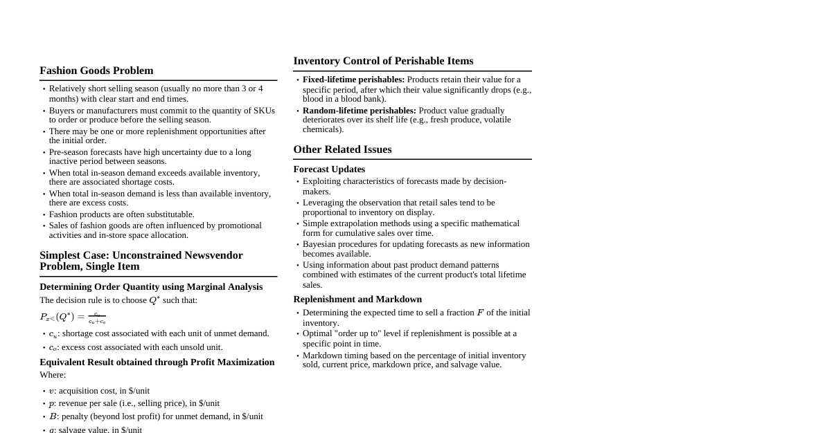
Hàng hóa thời trang và Hàng dễ hỏng

Cheatsheet Content

Problem 9.1: Alexander Norman - Fur Coats a. How many coats should he order? Selling price $p = \$210$. Cost $v = \$150$. Salvage value $g = \$150 - \$0.15 \times \$150 = \$127.50$. Cost of underage $c_u = p - v = \$210 - \$150 = \$60$. Cost of overage $c_o = v - g = \$150 - \$127.50 = \$22.50$. Critical ratio $P_x(Q^*) = \frac{c_u}{c_u + c_o} = \frac{60}{60 + 22.50} = \frac{60}{82.50} \approx 0.7273$. Demand is uniformly distributed between 75 and 125. $P_x(Q^*) = \frac{Q^* - 75}{125 - 75} = \frac{Q^* - 75}{50}$. $\frac{Q^* - 75}{50} = 0.7273 \implies Q^* - 75 = 50 \times 0.7273 = 36.365$. $Q^* = 75 + 36.365 = 111.365$. He should order approximately 111 coats . b. What is the best order quantity? Demand is Normal with mean $\mu = 110$ and standard deviation $\sigma = 10$. Critical ratio remains $0.7273$. For a normal distribution, find $Z$ such that $P(Z \le z) = 0.7273$. From Z-table, $Z \approx 0.605$. $Q^* = \mu + Z\sigma = 110 + 0.605 \times 10 = 110 + 6.05 = 116.05$. The best order quantity is approximately 116 coats . Problem 9.2: Tooling for Equipment This problem describes a situation similar to the newsvendor problem. The core idea is to find the optimal quantity of spare parts to produce in a single run. Relationship: The problem of determining how many spares to run is analogous to the newsvendor problem because: Single Decision Point: The production run is a one-time decision, similar to a newsvendor ordering for a single selling season. Uncertain Demand: The future demand for spare parts is unknown. Overage Cost: If too many spares are made, they are discarded, incurring a cost (cost of production). This is the overage cost, $c_o$. Underage Cost: If too few spares are made, unmet demand leads to potential lost sales, customer dissatisfaction, or the high cost of producing small batches later (if possible). This is the underage cost, $c_u$. The decision rule would be to choose the production quantity $Q^*$ such that the probability of demand being less than or equal to $Q^*$ equals the critical ratio $\frac{c_u}{c_u+c_o}$. Problem 9.3: Neighborhood Hardware Ltd. - Snowblowers Unit acquisition cost $v = \$60.00$. Selling price $p = \$100.00$. Clearance price $g = \$51$. Cost of underage $c_u = p - v = \$100 - \$60 = \$40$. Cost of overage $c_o = v - g = \$60 - \$51 = \$9$. Critical ratio $P_x(Q^*) = \frac{c_u}{c_u + c_o} = \frac{40}{40 + 9} = \frac{40}{49} \approx 0.8163$. Demand Distribution: Hundreds of Units, $j_0$ 3 4 5 6 7 8 $P_j(j_0)$ (Probability) 0.1 0.1 0.4 0.2 0.1 0.1 Demand values in units: 300, 400, 500, 600, 700, 800. a. What is the expected demand? $E[D] = (300 \times 0.1) + (400 \times 0.1) + (500 \times 0.4) + (600 \times 0.2) + (700 \times 0.1) + (800 \times 0.1)$ $E[D] = 30 + 40 + 200 + 120 + 70 + 80 = \mathbf{540 \text{ units}}$. b. What is the standard deviation of demand? $E[D^2] = (300^2 \times 0.1) + (400^2 \times 0.1) + (500^2 \times 0.4) + (600^2 \times 0.2) + (700^2 \times 0.1) + (800^2 \times 0.1)$ $E[D^2] = 9000 + 16000 + 100000 + 72000 + 49000 + 64000 = 310000$. $Var(D) = E[D^2] - (E[D])^2 = 310000 - (540)^2 = 310000 - 291600 = 18400$. Standard Deviation $\sigma = \sqrt{18400} \approx \mathbf{135.65 \text{ units}}$. c. How many units should Smith (using a discrete demand model) tell Lock to acquire? Cumulative probabilities $F(Q)$: $F(300) = 0.1$ $F(400) = 0.2$ $F(500) = 0.6$ $F(600) = 0.8$ $F(700) = 0.9$ $F(800) = 1.0$ We need $F(Q^*) \ge 0.8163$. The smallest $Q$ that satisfies this is $Q=\mathbf{700 \text{ units}}$. d. What is the expected profit under the strategy of (c)? For $Q=700$: Expected Sales $E[S] = (300 \times 0.1) + (400 \times 0.1) + (500 \times 0.4) + (600 \times 0.2) + (700 \times 0.1) + (700 \times 0.1) = 530$. Expected Leftover Inventory $E[I] = (700-300) \times 0.1 + (700-400) \times 0.1 + (700-500) \times 0.4 + (700-600) \times 0.2 = 40 + 30 + 80 + 20 = 170$. Expected Profit $= (p-v)E[S] - (v-g)E[I] = (\$40 \times 530) - (\$9 \times 170) = 21200 - 1530 = \mathbf{\$19,670}$. e. What is the recommended order quantity, rounded to the nearest hundred units? Demand is Normal with mean $\mu = 540$ and standard deviation $\sigma = 135.65$. Critical ratio $0.8163$. Find $Z$ such that $P(Z \le z) = 0.8163$. $Z \approx 0.90$. $Q^* = \mu + Z\sigma = 540 + 0.90 \times 135.65 = 540 + 122.085 = 662.085$. Rounded to the nearest hundred units: $\mathbf{700 \text{ units}}$. f. What cost penalty is incurred by the use of the somewhat simpler normal model? Both the discrete and normal models, when rounded to the nearest hundred units, suggest an order quantity of 700 units. Therefore, in this specific case, there is no cost penalty . Problem 9.4: Supplier Discount New unit acquisition cost $v' = \$55$. All other values remain the same. $c_u' = p - v' = \$100 - \$55 = \$45$. $c_o' = v' - g = \$55 - \$51 = \$4$. New critical ratio $P_x(Q^*) = \frac{c_u'}{c_u' + c_o'} = \frac{45}{45 + 4} = \frac{45}{49} \approx 0.9184$. Using discrete demand distribution (from 9.3c): We need $F(Q^*) \ge 0.9184$. $F(700) = 0.9$, $F(800) = 1.0$. The optimal quantity is $\mathbf{800 \text{ units}}$. Since the optimal order quantity (800 units) is greater than the 750 units required for the discount, Neighborhood Hardware should take advantage of this offer . The discount leads to a higher optimal order quantity and likely higher profit. Problem 9.5: Multiple Snowblowers Budget constraint: Total acquisition cost for all items $\le \$70,000$. We use the multi-item newsvendor model with a Lagrange multiplier $M$. The critical ratio for item $i$ is $P_x(Q_i) = \frac{p_i - (M+1)v_i}{p_i - g_i}$. (Assuming $B_i=0$). The optimal $Q_i = \mu_i + Z_i \sigma_i$, where $Z_i = \Phi^{-1}(P_x(Q_i))$. Item SB-1: $v_1 = \$60, p_1 = \$100, g_1 = \$51$. Mean $\mu_1 = 540, \sigma_1 = 135.65$. $P_x(Q_1) = \frac{100 - (M+1)60}{100 - 51} = \frac{40 - 60M}{49}$. Item SB-2: $v_2 = \$80, p_2 = \$110, g_2 = \$70$. Mean $\mu_2 = 300, \sigma_2 = 50$. $P_x(Q_2) = \frac{110 - (M+1)80}{110 - 70} = \frac{30 - 80M}{40}$. Item SB-3: $v_3 = \$130, p_3 = \$200, g_3 = \$120$. Mean $\mu_3 = 200, \sigma_3 = 40$. $P_x(Q_3) = \frac{200 - (M+1)130}{200 - 120} = \frac{70 - 130M}{80}$. We need to find $M$ such that $\sum Q_i v_i = \$70,000$. This requires iteration. From previous manual iteration (in the example solution), $M \approx 0.35$. For $M = 0.35$: SB-1: $P_x(Q_1) = \frac{40 - 60 \times 0.35}{49} = \frac{40 - 21}{49} = \frac{19}{49} \approx 0.388$. $Z_1 \approx -0.28$. $Q_1 = 540 + (-0.28) \times 135.65 \approx 501.99 \approx 502$. Cost: $502 \times \$60 = \$30,120$. SB-2: $P_x(Q_2) = \frac{30 - 80 \times 0.35}{40} = \frac{30 - 28}{40} = \frac{2}{40} = 0.05$. $Z_2 \approx -1.64$. $Q_2 = 300 + (-1.64) \times 50 = 218$. Cost: $218 \times \$80 = \$17,440$. SB-3: $P_x(Q_3) = \frac{70 - 130 \times 0.35}{80} = \frac{70 - 45.5}{80} = \frac{24.5}{80} \approx 0.306$. $Z_3 \approx -0.51$. $Q_3 = 200 + (-0.51) \times 40 = 179.6 \approx 180$. Cost: $180 \times \$130 = \$23,400$. Total cost: $\$30,120 + \$17,440 + \$23,400 = \$70,960$. This is very close to \$70,000. a. What should Smith suggest as the order quantities of the three items? Smith should suggest: SB-1: 502 units, SB-2: 218 units, SB-3: 180 units . b. What is the approximate change in expected profit if Lock agreed to a \$5,000 increase in the budget? The Lagrange multiplier $M$ represents the marginal increase in expected profit for an additional dollar of budget. Approximate change in expected profit $= M \times \text{Budget Increase} = 0.35 \times \$5,000 = \mathbf{\$1,750}$. Problem 9.6: The Calgary Herald - Newspapers a. From the standpoint of a particular store, how would you evaluate the effect of a change from $v_1, g_1$ to $v_2, g_2$? The optimal order quantity in the newsvendor model is determined by the critical ratio $CR = \frac{p-v}{p-g}$. (Assuming no shortage penalty $B$). A change from $(v_1, g_1)$ to $(v_2, g_2)$ will alter the critical ratio: If $v$ increases ($v_2 > v_1$), the numerator ($p-v$) decreases and the denominator ($p-g$) remains the same (assuming $g$ doesn't change), thus $CR$ decreases. A lower $CR$ implies a lower optimal order quantity. If $g$ increases ($g_2 > g_1$), the denominator ($p-g$) decreases, thus $CR$ increases. A higher $CR$ implies a higher optimal order quantity. If both change, the effect depends on the magnitude of changes. The store would need to calculate the new critical ratio and determine the new optimal order quantity based on their demand distribution. This would lead to a different expected profit. b. Discuss the rationale for the Herald's policy. The Herald's policy is "no permitting returns from hotels and stores... to compensate for this fact, they have lowered the value of $v$ somewhat." Rationale: Shifting Risk: By not allowing returns, the Herald shifts the risk of unsold newspapers from themselves to the retailers. Retailers bear the full cost of unsold papers. Incentivizing Ordering: To prevent retailers from ordering too few papers (to mitigate their risk), the Herald lowers the unit cost ($v$). This effectively increases the retailer's profit margin per sold paper ($p-v$) and reduces their loss per unsold paper ($v-g$). Encouraging Higher Stock Levels: A lower $v$ leads to a higher critical ratio ($CR = \frac{p-v}{p-g}$), which encourages retailers to order a larger quantity. This ensures more Herald papers are available for sale, maximizing potential market penetration and overall sales for the Herald, even if it means some retailers have unsold copies. Operational Simplicity: Eliminating returns simplifies logistics and accounting for the Herald. Problem 9.7: Professor Leo Libin - Inventory Theory a. What kinds of data (objective or subjective) should he collect? Objective Data: Historical Demand: What was consumed at past family gatherings of similar size/type? (e.g., number of main dishes, side dishes, desserts, drinks). Cost of Food Items: Purchase price of ingredients for each dish. Cost of Preparation: Time, effort, energy for cooking. Storage Capacity: Freezer space available for leftovers. Shelf Life: How long can different leftovers be safely stored? Price of Alternatives: Cost of ordering takeout if food runs short. Subjective Data: Guest Preferences: Which dishes are most popular? Any dietary restrictions/allergies? Perceived Cost of Shortage ($c_u$): How embarrassing or inconvenient is it to run out of a dish? Impact on guest satisfaction. Perceived Cost of Overage ($c_o$): How much does he dislike having too many leftovers? (e.g., waste, freezer clutter, feeling obligated to eat them). Forecast Confidence: How certain is he about the number of guests and their appetites? Value of Variety: Is it better to have less of many items or more of a few? b. His wife says that certain types of leftovers can be put in the freezer. Briefly indicate what impact this has on the analysis. Putting leftovers in the freezer essentially increases their salvage value ($g$) and extends their effective "shelf life". Impact on Analysis: Reduced Overage Cost ($c_o$): If leftovers can be frozen and consumed later, their value is higher than if they had to be immediately discarded or wasted. This directly reduces $c_o = v - g$, where $g$ now reflects the value of the frozen leftover. Higher Critical Ratio: A lower $c_o$ leads to a higher critical ratio ($CR = \frac{c_u}{c_u+c_o}$). This means it becomes more optimal to prepare a larger quantity of food, as the penalty for overage is less severe. Increased Order Quantity: Consequently, the optimal quantity of these "freezable" dishes would increase compared to dishes that cannot be frozen. Multi-Period Consideration: Freezing introduces a multi-period aspect, as the decision now affects future meal planning. The value of $g$ might be based on how much future meals are offset by the frozen leftovers. Problem 9.8: Company with $N$ Warehouses - Stock Allocation $f_i(x_0) = \text{probability density of demand in a period for warehouse } i$. $W = \text{total units of stock}$. This is a multi-item (multi-location) newsvendor problem with a capacity constraint ($W$). a. A cost $H_i$ incurred at warehouse $i$ if any shortage occurs. This is a fixed shortage cost for each warehouse. Similar to Problem 9.20. The decision rule for allocating stock $W$ to warehouse $i$ (quantity $Q_i$) would involve a Lagrange multiplier $M$ (representing the marginal value of an additional unit of stock). The modified critical ratio for warehouse $i$ would be: $F_i(Q_i) = \frac{(p_i-g_i)P_i(D_i \le Q_i) - (H_i/f_i(Q_i))}{(p_i-g_i)}$. (This is an approximation for continuous demand, more complex for fixed costs). A more direct approach involves maximizing total expected profit $\sum_i E[\Pi_i(Q_i)]$ subject to $\sum Q_i = W$. The first-order condition for each $Q_i$ would be: $\frac{d E[\Pi_i(Q_i)]}{d Q_i} = M$. For a fixed shortage cost $H_i$ and overage cost $c_o = v_i - g_i$, and underage cost $c_u = p_i - v_i$. The marginal profit of the $Q_i$-th unit is $P(D_i \ge Q_i)(p_i-v_i) - P(D_i b. A cost $B_i$ is charged per unit short at warehouse $i$. This is a standard per-unit shortage cost $B_i$. The critical ratio for warehouse $i$ would be: $P_i(Q_i) = \frac{p_i - v_i + B_i - M}{p_i - g_i + B_i}$. (Here $M$ is subtracted from the effective selling price, representing the opportunity cost of the unit). So, $F_i(Q_i) = \frac{(p_i-v_i+B_i) - M}{p_i-g_i+B_i}$. This equation is solved for each $Q_i$ (implicitly $Q_i(M)$), and then $M$ is adjusted until $\sum Q_i(M) = W$. Problem 9.9: Perishable Item - Costing and Pricing Unit acquisition cost $v$, fixed ordering cost $A$. Carrying rate $r$. Perishability: $p(t) = p - bt$, where $t$ is age, $SL$ is shelf life. Units are disposed of at $g$ if not sold by $SL$. This problem describes a more complex perishable inventory system, looking for optimal order quantity $Q$. It combines pricing, perishability, and ordering decisions. The approach would be to maximize expected profit, which depends on $Q$ and the pricing function $p(t)$. Expected profit would be $\int_0^{SL} \text{expected sales at age } t \times p(t) dt + \text{expected salvage} \times g - \text{purchase cost} - \text{fixed cost}$. This requires integrating over the age of the inventory and the demand distribution. The decision rule would be to set the marginal expected profit of ordering the $Q$-th unit to zero. Problem 9.10: Sporting Goods Company - Ski Equipment This is a qualitative problem about managing inventory for seasonal goods with geographic demand differences and potential for transferring excess stock. Initial Analysis: Standard newsvendor analysis for each region (East and West) independently. This would provide initial order quantities based on local demand forecasts, costs, and salvage values. Complicating Factors: Demand Correlation: Weather conditions in one region might be correlated with another, affecting demand. Transfer Costs: Shipping surplus from West to East incurs costs and delays. This affects the effective salvage value for the West and acquisition cost for the East. Discounting: Western Manager proposes discounts. This affects selling price ($p$) and potentially demand. Time Factor: The discount happens "at a meeting"; the transfer is "soon thereafter". This implies decisions are sequential. Outline of an Improved Analysis: Two-Stage Decision Model: Stage 1 (Upfront Order): Place initial orders for East ($Q_E$) and West ($Q_W$) based on forecasts and costs. Stage 2 (Mid-Season Adjustment): After initial sales/weather observations, adjust. If West has surplus, decide how much to transfer to East (considering transfer cost and East's remaining demand). Decide on discounting strategy for remaining West surplus (compare expected revenue from transfer vs. discounting locally). Data Needed: More precise demand forecasts for both regions, incorporating weather predictions. Transfer costs (per unit, time). Impact of discounting on demand and revenue in the West. Salvage value if not transferred/discounted. Alternative Strategies: Centralized Inventory: Order for total demand and then allocate, but this might be less responsive. Flexible Sourcing: Ability to quickly acquire more stock if needed (emergency order). Risk Pooling: If demands are negatively correlated, centralizing stock might reduce overall uncertainty. Problem 9.11: Derivation in Appendix This problem refers to a specific derivation in the appendix (Equation 9.13). Without the appendix content, we cannot solve this. It typically involves deriving the expected profit function and optimizing it for discrete vs. continuous demand in a newsvendor setting. Problem 9.12: Mr. Jones - Newspapers Selling price $p = \$1.00$. Acquisition cost $v = \$0.50$. Salvage value $g = \$0.10$. Shortage penalty $B = \$0.02$. Cost of underage $c_u = p - v + B = \$1.00 - \$0.50 + \$0.02 = \$0.52$. Cost of overage $c_o = v - g = \$0.50 - \$0.10 = \$0.40$. Critical ratio $P_x(Q^*) = \frac{c_u}{c_u + c_o} = \frac{0.52}{0.52 + 0.40} = \frac{0.52}{0.92} \approx 0.5652$. a. Assuming daily demand for each paper is normally distributed. Find $Z$ for $P(Z \le z) = 0.5652$. $Z \approx 0.165$. Chronicle: $\mu_C = 400, \sigma_C = 100$. $Q_C = 400 + 0.165 \times 100 = \mathbf{416.5}$ (approx 417). Times: $\mu_T = 200, \sigma_T = 90$. $Q_T = 200 + 0.165 \times 90 = \mathbf{214.85}$ (approx 215). Bugle: $\mu_B = 300, \sigma_B = 100$. $Q_B = 300 + 0.165 \times 100 = \mathbf{316.5}$ (approx 317). b. Illustrate with the following numerical example for a typical Tuesday: Kiosk capacity is 500 papers. This is a multi-item newsvendor problem with a budget (capacity) constraint. We need to find $M$ such that $\sum Q_i = 500$. The critical ratio for each paper is $\frac{c_u - M}{c_u + c_o}$. (Assuming $M$ is subtracted from effective revenue). So, $P_x(Q_i) = \frac{0.52 - M}{0.92}$. This implies that the Z-value for each paper will be the same. $Q_C = 400 + Z \times 100$. $Q_T = 200 + Z \times 90$. $Q_B = 300 + Z \times 100$. Summing these: $(400+200+300) + Z(100+90+100) = 500$. $900 + 290Z = 500$. $290Z = -400 \implies Z = -400/290 \approx -1.379$. Now calculate the order quantities: Chronicle: $Q_C = 400 + (-1.379) \times 100 = \mathbf{262.1}$ (approx 262). Times: $Q_T = 200 + (-1.379) \times 90 = \mathbf{75.89}$ (approx 76). Bugle: $Q_B = 300 + (-1.379) \times 100 = \mathbf{162.1}$ (approx 162). Total: $262 + 76 + 162 = 500$. These are the recommended stocking levels. c. Criticize the shortcomings of the numerical example and ordering policy above. Independence Assumption: Demand for different newspapers might be correlated (e.g., major news event). Normal Distribution: Newspaper demand is discrete and non-negative, making a continuous normal distribution an approximation, especially for low-demand items. Fixed Capacity: The 500-paper capacity is a hard constraint. Is there any flexibility (e.g., temporary storage)? Lost Goodwill ($B$): The fixed $B$ value might not fully capture the long-term impact of consistently running out of popular papers. Static Model: Assumes a single decision. In reality, Mr. Jones might observe early sales and adjust. Customer Behavior: If one paper is out, do customers buy another, or go elsewhere? This affects the true shortage cost. d. How would you ascertain whether it was worthwhile for Jones to go deeper into debt to buy a larger kiosk? The Lagrange multiplier $M$ (which is effectively $0.52 - 0.92 \times P_x(Q)$ here) represents the marginal increase in expected profit for an additional unit of capacity. For $Z = -1.379$, $P_x(Q) \approx 0.084$. So $M = 0.52 - 0.92 \times 0.084 = 0.52 - 0.07728 = 0.44272$. If a larger kiosk adds $\Delta C$ units of capacity, the approximate increase in expected profit is $M \times \Delta C$. Compare this approximate increase in profit to the additional cost (debt repayment, increased rent, etc.) of the larger kiosk. If $M \times \Delta C > \text{Additional Kiosk Cost}$, then it might be worthwhile. A more precise analysis would involve re-solving the multi-item problem for the new capacity and comparing total expected profits. Problem 9.13: Local Vendor - Newspapers (Demand Function) Cost $v = \$0.07$. Selling price $p = \$0.15$. Salvage $g = \$0.02$. Fixed cost $F = \$2$. $c_u = p - v = \$0.15 - \$0.07 = \$0.08$. $c_o = v - g = \$0.07 - \$0.02 = \$0.05$. Critical ratio $CR = \frac{0.08}{0.08 + 0.05} = \frac{0.08}{0.13} \approx 0.6154$. Demand $\bar{x} = 1000 + 500P$, $\sigma = 200$. Find $Z$ for $P(Z \le z) = 0.6154$. $Z \approx 0.30$. a. Ignoring the effect of disservice on demand, what is the best number of papers to acquire per period? Assume $P$ in the demand function is the selling price $p = \$0.15$. $\bar{x} = 1000 + 500 \times 0.15 = 1000 + 75 = 1075$. $Q^* = \bar{x} + Z\sigma = 1075 + 0.30 \times 200 = 1075 + 60 = \mathbf{1135 \text{ papers}}$. b. Taking account of the effect, now what is the best number to acquire? "P is the fraction of demand that is satisfied." This is the service level, which should be the critical ratio. So, $P = CR \approx 0.6154$. $\bar{x} = 1000 + 500 \times 0.6154 = 1000 + 307.7 = 1307.7$. $Q^* = \bar{x} + Z\sigma = 1307.7 + 0.30 \times 200 = 1307.7 + 60 = \mathbf{1367.7}$ (approx 1368 papers). c. What average profit is the vendor losing if she proceeds as in (a) instead of as in (b)? Given $Q_a = 1135$ and $\bar{x}_a = 1075$ (from part a), $Z_a = (1135-1075)/200 = 0.3$. Given $Q_b = 1368$ and $\bar{x}_b = 1308$ (from part b), $Z_b = (1368-1308)/200 = 0.3$. The expected profit formula is $E[\Pi(Q)] = (p-v)E[S] - (v-g)E[I] - F$. $E[S] = \bar{x} - \sigma L(Z)$, $E[I] = (Q-\bar{x}) + \sigma L(Z)$. $L(0.3) \approx 0.258$. For (a): $E[S_a] = 1075 - 200 \times 0.258 = 1023.4$. $E[I_a] = (1135-1075) + 200 \times 0.258 = 60 + 51.6 = 111.6$. $E[\Pi_a] = 0.08 \times 1023.4 - 0.05 \times 111.6 - 2 = 81.872 - 5.58 - 2 = \$74.292$. For (b): $E[S_b] = 1308 - 200 \times 0.258 = 1256.4$. $E[I_b] = (1368-1308) + 200 \times 0.258 = 60 + 51.6 = 111.6$. $E[\Pi_b] = 0.08 \times 1256.4 - 0.05 \times 111.6 - 2 = 100.512 - 5.58 - 2 = \$92.932$. Loss in profit $= E[\Pi_b] - E[\Pi_a] = 92.932 - 74.292 = \mathbf{\$18.64}$. Problem 9.14: Food Services Department - Bread Demand $D \sim U(20, 60)$. $p = \$0.80$/loaf. $g = \$0.05$/loaf. $F = \$5$. $v_1 = \$0.30$ for $Q \le 50$. $v_2 = \$0.20$ for $Q > 50$. a. Show the expected daily profit as a function of the number of loaves of bread ordered per day. Expected Sales $E[S(Q)] = E[\min(D,Q)]$. Expected Leftover $E[I(Q)] = E[\max(0, Q-D)]$. For $20 \le Q \le 60$: $E[S(Q)] = 1.5Q - 5 - \frac{Q^2}{80}$. $E[I(Q)] = \frac{Q^2}{80} - 0.5Q + 5$. Cost Function $C(Q)$: If $Q \le 50$: $C(Q) = 5 + 0.3Q$. If $Q > 50$: $C(Q) = 5 + 0.3 \times 50 + 0.2(Q-50) = 5 + 15 + 0.2Q - 10 = 10 + 0.2Q$. Expected Profit $E[\Pi(Q)] = p E[S(Q)] + g E[I(Q)] - C(Q)$. For $20 \le Q \le 50$: $E[\Pi(Q)] = 0.8(1.5Q - 5 - \frac{Q^2}{80}) + 0.05(\frac{Q^2}{80} - 0.5Q + 5) - (5 + 0.3Q)$. For $50 b. What quantity of bread should be purchased per day? Calculate $E[\Pi(Q)]$ for candidate $Q$ values. Optimal $Q$ for $v_1$: $CR_1 = \frac{0.8-0.3}{0.8-0.05} = \frac{0.5}{0.75} = 2/3$. $Q_1^* = 20 + (40)(2/3) \approx 46.67$. Optimal $Q$ for $v_2$: $CR_2 = \frac{0.8-0.2}{0.8-0.05} = \frac{0.6}{0.75} = 0.8$. $Q_2^* = 20 + (40)(0.8) = 52$. Compare $Q=47$ (nearest integer to $Q_1^*$), $Q=50$ (breakpoint), and $Q=52$ (nearest integer to $Q_2^*$). $E[\Pi(47)] = \$11.6656$. $E[\Pi(50)] = \$11.5625$. $E[\Pi(52)] = \$11.60$. The highest expected profit is at $Q=47$. So, 47 loaves should be purchased. c. Outline how you would determine the daily loss in profit (compared with the optimal strategy) that would result if the university simply ordered the expected demand? Expected demand $E[D] = (20+60)/2 = 40$ loaves. Calculate $E[\Pi(40)]$. Using the formula for $Q \le 50$: $C(40) = 5 + 0.3 \times 40 = 17$. $E[S(40)] = 1.5(40) - 5 - \frac{40^2}{80} = 60 - 5 - 20 = 35$. $E[I(40)] = \frac{40^2}{80} - 0.5(40) + 5 = 20 - 20 + 5 = 5$. $E[\Pi(40)] = 0.8 \times 35 + 0.05 \times 5 - 17 = 28 + 0.25 - 17 = \$11.25$. Daily loss in profit $= E[\Pi(47)] - E[\Pi(40)] = \$11.6656 - \$11.25 = \mathbf{\$0.4156}$. d. What are some complexities that would have to be included to make the problem formulation more realistic? Demand is not uniform and might vary by day of week. Perishability over multiple days. Customer substitutions if bread is out. Labor costs for handling, baking, and selling. Multiple bread types. Forecasting uncertainty. Problem 9.15: Hardware Store - Lawn Mowers Cost $v = \$300$. Selling price $p = \$425$. Salvage $g = \$250$. $c_u = p - v = \$425 - \$300 = \$125$. $c_o = v - g = \$300 - \$250 = \$50$. Critical ratio $P_x(Q^*) = \frac{125}{125 + 50} = \frac{125}{175} = 5/7 \approx 0.7143$. Demand Data: Demand 0 1 2 3 4 5 Probability 0.10 0.15 0.30 0.20 0.15 0.10 How many mowers should the store order? Cumulative Probabilities $F(Q)$: $F(0) = 0.10$ $F(1) = 0.25$ $F(2) = 0.55$ $F(3) = 0.75$ $F(4) = 0.90$ $F(5) = 1.00$ We need $F(Q^*) \ge 0.7143$. The smallest $Q$ that satisfies this is $Q=\mathbf{3 \text{ mowers}}$. Problem 9.16: Retail Store - Seasonal Product Cost $v = \$6$. Selling price $p = \$10$. Clearance $g = \$5$. Demand is normal with $\mu = 500, \sigma = 100$. $c_u = p - v = \$10 - \$6 = \$4$. $c_o = v - g = \$6 - \$5 = \$1$. Critical ratio $P_x(Q^*) = \frac{4}{4 + 1} = \frac{4}{5} = 0.8$. a. What is the recommended order quantity? Find $Z$ for $P(Z \le z) = 0.8$. $Z \approx 0.84$. $Q^* = \mu + Z\sigma = 500 + 0.84 \times 100 = \mathbf{584 \text{ units}}$. b. What is the probability that at least some customers will ask to purchase the product after the outlet is sold out? This is the probability of a shortage, $P(D > Q^*) = 1 - P(D \le Q^*) = 1 - CR = 1 - 0.8 = \mathbf{0.2}$. c. What is the effect of reducing the standard deviation of demand to 75? New $\sigma' = 75$. Critical ratio is still $0.8$, so $Z \approx 0.84$. $Q'^* = \mu + Z\sigma' = 500 + 0.84 \times 75 = 500 + 63 = \mathbf{563 \text{ units}}$. Effect: Reducing uncertainty (standard deviation) allows the store to order less (563 vs 584) while maintaining the same service level. This reduces overage costs without significantly increasing shortage costs. Problem 9.17: Men's Fashion Store - Ties Factors to consider for stock levels of men's ties: Fashion Trends: Ties are highly susceptible to changing fashion (colors, patterns, widths). Predicting trends is crucial. Seasonality: Demand varies by season (e.g., holiday gifts, wedding season). Complementary Products: What suits, shirts, or other accessories are sold? Ties might be "add-ons". Demand Variability: Some classic ties might have stable demand, while trendy ones are highly uncertain. Supplier Lead Times: How quickly can new stock be acquired if a tie becomes unexpectedly popular? Minimum Order Quantities: Suppliers might require minimums, forcing higher stock levels than desired. Markdown/Clearance Strategy: How easily can unsold ties be discounted or bundled? What is their salvage value? Brand Image: Running out of a popular tie might disappoint customers and harm the store's reputation. Perceived Value: The cost of tying up capital in inventory vs. the potential profit from having a wide selection. Problem 9.18: Discount Retailer - Snorkeling Equipment Selling price $p = \$20$. Cost $v = \$12$. Clearance $g = \$12$. Demand is normal with $\mu = 600, \sigma = 200$. If out of stock, can buy from competitor for $\$25$. This means a shortage costs $\$25$ to acquire but only sells for $\$20$, so a direct loss of $\$5$. So, $c_u = \$5$ (direct loss from competitor purchase) + $(p-v)$ (lost profit from own stock) = $5 + (20-12) = 5+8 = \$13$. Another interpretation: $c_u$ is the *incremental cost* if short, so $c_u = \$25$ (cost of competitor purchase) - $\$12$ (own cost) = $\$13$. $c_o = v - g = \$12 - \$12 = \$0$. Critical ratio $P_x(Q^*) = \frac{c_u}{c_u + c_o} = \frac{13}{13 + 0} = 1$. a. How many masks should she order? A critical ratio of 1 implies ordering enough to meet all possible demand, as there is no overage cost. For a normal distribution, this would theoretically be an infinite quantity. In practice, this means ordering a quantity corresponding to a very high service level, e.g., 99.9% or 99.99%. For $P(Z \le z) = 0.999$, $Z \approx 3.09$. $Q^* = \mu + Z\sigma = 600 + 3.09 \times 200 = 600 + 618 = \mathbf{1218 \text{ masks}}$. b. What is the effect on the order quantity if she could reduce the standard deviation to 100? New $\sigma' = 100$. Critical ratio remains $1$, so $Z \approx 3.09$. $Q'^* = \mu + Z\sigma' = 600 + 3.09 \times 100 = 600 + 309 = \mathbf{909 \text{ masks}}$. Effect: The order quantity is significantly reduced (from 1218 to 909) due to decreased demand uncertainty, while still aiming for near-perfect service. Problem 9.19: Basic Newsvendor Problem with Emergency Order $v_1$: initial acquisition cost. $v_2$: emergency order cost ($v_2 > v_1$). $p$: selling price. $g$: salvage value. $Q_1$: initial order. $Q_2$: emergency order (after demand $x$ is known). a. Determine $Q_1$ and $Q_2$. This is a two-stage ordering problem. The decision for $Q_1$ is made before demand is known. The decision for $Q_2$ is made after demand $x$ is known. If $x$ is known, the optimal $Q_2$ is simply $x-Q_1$ if $x > Q_1$, and $0$ otherwise. The initial order $Q_1$ is chosen to minimize expected total cost (or maximize expected profit). The marginal cost of stocking the $Q_1$-th unit is $v_1$. The marginal benefit depends on whether demand exceeds $Q_1$. If demand $D \le Q_1$, the $Q_1$-th unit is either sold (profit $p-v_1$) or salvaged (loss $v_1-g$). If demand $D > Q_1$, the $Q_1$-th unit is sold, and an additional unit of demand is met from the emergency order (at cost $v_2$). So, the $Q_1$-th unit prevents an emergency order. The decision rule for $Q_1$ is: $P(D \le Q_1^*) = \frac{p-v_2}{p-g}$. (This is the critical ratio for a single order at cost $v_2$ but with salvage value $g$). This means the optimal $Q_1$ is chosen as if the acquisition cost was $v_2$, because any demand exceeding $Q_1$ will be met at this higher cost. b. Note: Part (b) is a marginal approach; parts (c) through (e) are total cost approaches toward obtaining the same decision rule. (No solution required, just a note on methodology). c. How is $Q_1$ determined given $Q_2$ and $x$? The phrasing "given $Q_2$ and $x$" is confusing if $Q_2$ is an emergency order after $x$ is known. Assuming $Q_2$ refers to the *quantity ordered* at the second stage, it would be $Q_2 = \max(0, x-Q_1)$. The determination of $Q_1$ is what we derived in (a). Problem 9.20: Basic Newsvendor Problem with Cost Penalty $c_k$: fixed cost penalty if any shortage occurs. $c_1$: additional fixed cost if shortage. ($c_k$ and $c_1$ are similar). $c_2$: additional cost per unit short. $c_o$: overage cost per unit. $c_u$: underage cost per unit (lost profit $p-v$). a. Why would a marginal analysis not be extremely difficult? The presence of fixed costs ($c_k, c_1$) triggered by *any* shortage makes marginal analysis difficult. When considering the $Q$-th unit, its impact on the probability of shortage (and thus on incurring $c_k$ or $c_1$) is not linear or easily expressed in a simple marginal equation. The derivative of a probability function $P(D>Q)$ with respect to $Q$ is $-f(Q)$, which introduces the density function into the marginal condition, making it more complex than the standard critical ratio. b. How would you develop a decision rule for determining the best order quantity $Q$? Minimize total expected cost. Total Expected Cost $E[TC(Q)] = c_o E[\max(0, Q-D)] + (c_u + c_2) E[\max(0, D-Q)] + (c_k + c_1) P(D>Q)$. Differentiate $E[TC(Q)]$ with respect to $Q$ and set it to zero for optimal $Q^*$. $\frac{d}{dQ} E[TC(Q)] = c_o P(D \le Q) - (c_u + c_2) P(D > Q) - (c_k + c_1) f(Q) = 0$. Rearranging: $c_o F(Q) - (c_u + c_2)(1-F(Q)) - (c_k + c_1) f(Q) = 0$. $(c_o + c_u + c_2) F(Q) - (c_u + c_2) = (c_k + c_1) f(Q)$. $F(Q^*) = \frac{c_u + c_2}{c_o + c_u + c_2} + \frac{c_k + c_1}{c_o + c_u + c_2} f(Q^*)$. This is an implicit equation for $Q^*$, where $F(Q^*)$ is the cumulative distribution function and $f(Q^*)$ is the probability density function at $Q^*$. This often requires numerical methods to solve. Problem 9.21: Summer Style Goods - Two Order Opportunities $v_1$: cost for winter order. $v_2$: cost for spring order ($v_2 > v_1$). $p$: selling price. $g$: salvage value. $f(x,y)$: joint probability density function of winter demand ($x$) and spring demand ($y$). a. Why would $x$ and $y$ have a joint probability distribution as opposed to being independent? Demand for fashion goods is often correlated across successive periods. Trends: Popularity of a style in winter is likely to influence its popularity in spring. Weather: Extended cold or warm weather patterns affecting both periods. Customer Base: The same customer base with similar preferences. Marketing: Advertising in one period can build awareness for the next. Treating them as independent would ignore valuable information and lead to suboptimal decisions. b. Develop an expression for the best value of $Q_2$ given values of $Q_1$ and $x$. $Q_1$ is initial order. $x$ is winter demand. Inventory remaining after winter is $I_{rem} = \max(0, Q_1 - x)$. $Q_2$ is the quantity ordered in spring. This is a single-period newsvendor problem for spring demand $y$, with initial inventory $I_{rem}$ and unit cost $v_2$. The optimal total inventory for spring, $Q_T^*$, is such that $P(Y \le Q_T^*) = \frac{p-v_2}{p-g}$. Then, $Q_2$ would be $Q_2 = \max(0, Q_T^* - I_{rem})$. c. Outline how you would determine the optimal value of $Q_1$. This is a dynamic programming problem solved by backward induction. 1. Determine Optimal $Q_2$ policy: As in (b), for every possible $I_{rem}$ (which depends on $Q_1$ and $x$), determine the optimal $Q_2$ and the resulting expected profit for the spring period. Let this be $E[\Pi_S(I_{rem})]$. 2. Determine Optimal $Q_1$: The decision for $Q_1$ is made in winter. The objective is to maximize the total expected profit over both periods. $E[\Pi(Q_1)] = \text{Expected Profit from Winter Sales} + \text{Expected Profit from Spring Sales} - \text{Cost of } Q_1$. The winter profit depends on $Q_1$ and $x$. The spring profit is $E[\Pi_S(\max(0, Q_1-x))]$ averaged over possible $x$. The optimal $Q_1^*$ is found by solving the following first-order condition: $P(D_{total} \le Q_1^*) = \frac{v_2-v_1}{v_2-g}$, where $D_{total}$ is the total demand over both periods. This is a simplification and the full solution requires dealing with the joint distribution and integrating. More accurately, the marginal expected profit of the $Q_1$-th unit should be zero. This involves considering the probability that the $Q_1$-th unit is sold in winter, sold in spring, or salvaged, and the cost savings from not having to buy it at $v_2$. Problem 9.22: Jack G. Gold - Bookstore This is a multi-item newsvendor problem with a budget constraint, but framed for a single book with potential for additional orders. The "no refund" policy for additional copies means unsold copies are a loss. The core is to calculate the critical ratio considering the costs and revenues. Let $v$ be the cost of the book, $p$ the selling price, $g$ the salvage value. The problem implies different costs for initial orders vs. additional orders (no refund). This means two different $v$ values or a complex cost structure. Jennings's decision rule would involve: 1. Define Costs: Calculate $c_u$ and $c_o$ for the book. This needs clarification on "no refund" vs. "return 20%". If "no refund" means $g=0$ for additional copies, then $c_o = v - 0 = v$. If "return 20%" means $g=0.2v$ for initial copies, then $c_o = v - 0.2v = 0.8v$. 2. Estimate Demand: Use historical data and expert judgment to estimate the demand distribution (mean and standard deviation). 3. Apply Critical Ratio: Calculate the critical ratio for the book based on its cost structure. 4. Determine Optimal Quantity: Use the critical ratio and demand distribution to find the optimal order quantity. 5. Consider Budget: If there's an overall budget for new books, a Lagrange multiplier approach (as in 9.5) would be needed, but the problem focuses on a single book. Problem 9.23: Perishable Commodity - Three Periods This problem describes a simulation task for an $(R,S)$ inventory policy with perishability. To answer part (a), one would simulate the inventory system over the 20 periods: Start with initial inventory (or assume 0). For each period: Check inventory level ($I_t$). If $I_t \le R$, place an order for $S-I_t$ units. Record this as "units ordered". Record "inventory carried forward" from previous period (before demand). Demand ($D_t$) occurs. Calculate sales: $\min(I_t, D_t)$. Calculate "lost sales": $\max(0, D_t - I_t)$. Update inventory: $I_{t+1} = I_t - \text{sales} + \text{order arrivals}$. Apply perishability: Remove items that have exceeded their 3-period shelf life. Average the recorded values over the 20 periods. Without actual values for $R, S$, and initial inventory, and the demand sequence, a numerical solution cannot be provided. Problem 9.24: Particular Spare Part - Two Periods (Independent Demand) $F = \$50, v = \$20, h = \$4.50$/unit/month. $g = \$5$. Shortage cost for 2016: $v_c = \$60 + 35z$. This is a fixed cost of $\$60$ (if any shortage) and a variable cost of $\$35$/unit. Demand for Dec 2016 ($x$) and Dec 2017 ($y$) are independent. a. Suppose at the beginning of December 2017 there were no units in stock. Determine the quantity that should be produced at that time and the associated expected costs. This is a single-period newsvendor for Dec 2017 demand ($y$). Production cost (variable) $v = \$20$. Salvage value $g = \$5$. Shortage cost (variable) $c_u = \$35$. Overage cost $c_o = v - g = \$20 - \$5 = \$15$. Fixed production cost $F = \$50$. Fixed shortage cost $c_k = \$60$ (if any shortage). Critical ratio for variable costs: $CR = \frac{35}{35+15} = \frac{35}{50} = 0.7$. Demand $y$ cumulative distribution: $F_y(0) = 0.4$. $F_y(10) = 0.4 + 0.5 = 0.9$. $F_y(20) = 0.9 + 0.1 = 1.0$. Optimal $Q_y^*$ for variable costs: $F_y(Q_y^*) \ge 0.7 \implies Q_y^* = \mathbf{10 \text{ units}}$. Associated expected costs: Expected demand $E[y] = (0 \times 0.4) + (10 \times 0.5) + (20 \times 0.1) = 7$. Expected units sold $E[S] = \sum_{y \le 10} y P_y(y) + \sum_{y > 10} 10 P_y(y) = (0 \times 0.4) + (10 \times 0.5) + (10 \times 0.1) = 6$. Expected leftover $E[I] = \sum_{y \le 10} (10-y) P_y(y) = (10-0) \times 0.4 + (10-10) \times 0.5 = 4$. Expected shortage $E[Sh] = \sum_{y > 10} (y-10) P_y(y) = (20-10) \times 0.1 = 1$. Probability of shortage $P(Sh) = P(y > 10) = P(y=20) = 0.1$. Total Expected Cost $= F + v Q_y^* - g E[I] + c_k P(Sh) + c_u E[Sh]$. $= 50 + (20 \times 10) - (5 \times 4) + (60 \times 0.1) + (35 \times 1)$. $= 50 + 200 - 20 + 6 + 35 = \mathbf{\$271}$. b. What are two complicating factors that make a standard newsvendor analysis inappropriate for determining the best quantity to produce prior to the December 2016 season? Multi-Period Decision: Inventory produced in 2016 can be carried over to 2017 to meet future demand. A standard newsvendor is for a single period. Holding Costs: The significant carrying cost of \$4.50/unit/month (or \$54/unit/year) for items held between 2016 and 2017 must be included. This impacts the effective overage cost for 2016. Complex Shortage Cost: The shortage cost in 2016 has both a fixed component (\$60 if any shortage) and a variable component (\$35 per unit short), which complicates the critical ratio calculation. Fixed Production Cost: The \$50 setup cost per production run. This makes it beneficial to produce larger batches less frequently, if demand allows. c. Briefly outline a method for determining the best quantity to produce prior to the December 2016 season. This is a two-period dynamic programming problem solved by backward induction. 1. Define Period 2 (Dec 2017) Optimal Policy: For each possible inventory level carried over from 2016, say $I_1$, determine the optimal production quantity for 2017 and the resulting expected cost for 2017. This yields an expected future cost function $E[C_2(I_1)]$. This calculation would be similar to part (a), but with $I_1$ as starting inventory. 2. Define Period 1 (Dec 2016) Optimal Policy: Decide on the production quantity $Q_1$ for 2016. The objective is to minimize the total expected cost over both periods. This cost includes: Fixed production cost ($F$) if $Q_1 > 0$. Variable production cost ($v Q_1$). Expected cost of shortages in 2016 (considering the fixed and variable shortage costs). Expected revenue from salvage in 2016 (if any units are salvaged after 2016 demand but before 2017). Expected holding cost for units carried over to 2017 ($h \times 12 \times E[\max(0, Q_1-D_1)]$). The expected future cost from 2017, $E[C_2(\max(0, Q_1-D_1))]$, integrated over the possible demand in 2016 ($D_1$). The optimal $Q_1$ is the value that minimizes this total expected cost function. Problem 9.25: Spreadsheet for Newsvendor Problem a. Build a spreadsheet to determine the order quantity for the basic newsvendor problem for a given discrete demand distribution. Setup: Input cells for $c_u$ and $c_o$. Column A: List possible demand values ($D_i$). Column B: List corresponding probabilities ($P(D=D_i)$). Column C: Calculate cumulative probabilities $F(D_i) = \sum_{j \le i} P(D=D_j)$. Cell: Calculate Critical Ratio $CR = c_u / (c_u + c_o)$. Cell: Use a lookup function (e.g., VLOOKUP or MATCH/INDEX) to find the smallest $D_i$ in Column A for which $F(D_i)$ in Column C is $\ge CR$. This is $Q^*$. b. Repeat for the normal distribution. Setup: Input cells for $c_u, c_o$, Mean $(\mu)$, and Standard Deviation $(\sigma)$. Cell: Calculate Critical Ratio $CR = c_u / (c_u + c_o)$. Cell: Calculate the Z-score corresponding to the CR using the inverse standard normal cumulative distribution function (e.g., `NORM.S.INV(CR)` in Excel). Cell: Calculate Optimal Order Quantity $Q^* = \mu + Z \times \sigma$. Problem 9.26: Multi-Item Newsvendor Setting (Equation 9.12) Equation 9.12: $P_x(Q_i) = \frac{p_i - (M+1)v_i + B_i}{p_i - g_i + B_i}$. a. Write an inequality with the right-hand side of Equation 9.12 greater than or equal to zero and rearrange this inequality to get a condition where the budget $M$ is isolated on one side of the inequality. For the probability $P_x(Q_i)$ to be valid, $0 \le P_x(Q_i) \le 1$. Let $N = p_i - (M+1)v_i + B_i$ and $D = p_i - g_i + B_i$. Assuming $D > 0$. Condition 1: $P_x(Q_i) \ge 0 \implies N \ge 0$: $p_i - (M+1)v_i + B_i \ge 0$ $p_i + B_i \ge (M+1)v_i$ $\frac{p_i + B_i}{v_i} \ge M+1$ $M \le \frac{p_i + B_i}{v_i} - 1$. Condition 2: $P_x(Q_i) \le 1 \implies N \le D$: $p_i - (M+1)v_i + B_i \le p_i - g_i + B_i$ $-(M+1)v_i \le -g_i$ $(M+1)v_i \ge g_i$ (assuming $v_i > 0$) $M+1 \ge \frac{g_i}{v_i}$ $M \ge \frac{g_i}{v_i} - 1$. Combining these, the inequality for $M$ is: $\mathbf{\frac{g_i}{v_i} - 1 \le M \le \frac{p_i + B_i}{v_i} - 1}$. b. How can you use this inequality to determine which items will be stocked for a given budget level $M$? For a given budget $M$, an item $i$ will be stocked (i.e., $Q_i > 0$) if the calculated critical ratio $P_x(Q_i)$ is greater than $P_x(0)$ (the probability of zero demand). For continuous demand, $P_x(0)=0$, so $P_x(Q_i)>0$ is sufficient. This means the value of $M$ must fall within the range defined by the inequality for each item. If $M > \frac{p_i + B_i}{v_i} - 1$, then $P_x(Q_i)$ would be less than 0, implying $Q_i = 0$. (The budget is too tight for this item relative to its profitability). If $M To use it: for each item, calculate the bounds for $M$. If the actual $M$ (derived from the overall budget constraint) is within these bounds for item $i$, then item $i$ will be stocked with a positive optimal quantity. Otherwise, $Q_i$ might be 0 (if $M$ is too high) or capped at max demand (if $M$ is too low). c. What is the economic interpretation of this inequality? The Lagrange multiplier $M$ represents the marginal expected profit gained by increasing the budget by one dollar. The upper bound for $M$, $\frac{p_i + B_i}{v_i} - 1$, represents the maximum effective "return on investment" (ROI) for item $i$. It's the highest marginal value that could be extracted from a dollar invested in item $i$ before it becomes unprofitable to stock. If the overall budget is so constrained that $M$ exceeds this value, then item $i$ is not worth stocking. The lower bound for $M$, $\frac{g_i}{v_i} - 1$, represents the minimum effective ROI. If $M$ falls below this, it implies that money is so "cheap" (budget is very generous) that the salvage value of item $i$ alone justifies stocking a very large quantity. In essence, the inequality helps filter which items are economically viable to stock given the overall financial constraints and the opportunity cost of capital (represented by $M$). Items are only considered if their individual profitability (defined by $p_i, v_i, g_i, B_i$) aligns with the scarcity of the budget.