Statistics Cheatsheet

Cheatsheet Content

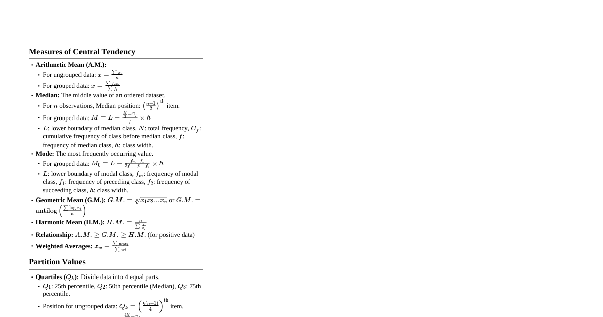
1. Descriptive Statistics 1.1 Measures of Central Tendency Mean (Average): $\bar{x} = \frac{1}{n} \sum_{i=1}^n x_i$ Median: Middle value when data is ordered. If $n$ is even, average of two middle values. Mode: Most frequent value in the dataset. 1.2 Measures of Dispersion Range: Max value - Min value. Variance: Population Variance: $\sigma^2 = \frac{1}{N} \sum_{i=1}^N (x_i - \mu)^2$ Sample Variance: $s^2 = \frac{1}{n-1} \sum_{i=1}^n (x_i - \bar{x})^2$ Standard Deviation: $\sigma = \sqrt{\sigma^2}$ (population), $s = \sqrt{s^2}$ (sample). Interquartile Range (IQR): $Q_3 - Q_1$. 1.3 Skewness & Kurtosis Skewness: Measures asymmetry of the probability distribution. Positive Skew: Tail on the right (Mean > Median). Negative Skew: Tail on the left (Mean Kurtosis: Measures "tailedness" of the distribution. Leptokurtic: Heavy tails, sharp peak. Mesokurtic: Normal tails (e.g., normal distribution). Platykurtic: Light tails, flatter peak. 2. Probability 2.1 Basic Concepts Probability of Event A: $P(A) = \frac{\text{Number of favorable outcomes}}{\text{Total number of outcomes}}$ Complement Rule: $P(A^c) = 1 - P(A)$ Addition Rule: $P(A \cup B) = P(A) + P(B) - P(A \cap B)$ Mutually Exclusive Events: $P(A \cap B) = 0 \implies P(A \cup B) = P(A) + P(B)$ Conditional Probability: $P(A|B) = \frac{P(A \cap B)}{P(B)}$ Multiplication Rule: $P(A \cap B) = P(A|B)P(B) = P(B|A)P(A)$ Independent Events: $P(A \cap B) = P(A)P(B) \implies P(A|B) = P(A)$ 2.2 Bayes' Theorem $P(A|B) = \frac{P(B|A)P(A)}{P(B)}$ 3. Probability Distributions 3.1 Discrete Distributions Bernoulli: $P(X=k) = p^k (1-p)^{1-k}$ for $k \in \{0, 1\}$. Mean $p$, Variance $p(1-p)$. Binomial: $P(X=k) = \binom{n}{k} p^k (1-p)^{n-k}$. Mean $np$, Variance $np(1-p)$. Poisson: $P(X=k) = \frac{\lambda^k e^{-\lambda}}{k!}$. Mean $\lambda$, Variance $\lambda$. 3.2 Continuous Distributions Uniform: $f(x) = \frac{1}{b-a}$ for $a \le x \le b$. Mean $\frac{a+b}{2}$, Variance $\frac{(b-a)^2}{12}$. Normal (Gaussian): $f(x) = \frac{1}{\sigma \sqrt{2\pi}} e^{-\frac{1}{2}(\frac{x-\mu}{\sigma})^2}$. Mean $\mu$, Variance $\sigma^2$. Standard Normal: $Z = \frac{X-\mu}{\sigma}$. Mean 0, Variance 1. Exponential: $f(x) = \lambda e^{-\lambda x}$ for $x \ge 0$. Mean $\frac{1}{\lambda}$, Variance $\frac{1}{\lambda^2}$. 4. Sampling & Estimation 4.1 Sampling Distributions Central Limit Theorem (CLT): For large $n$, the sampling distribution of the sample mean $\bar{X}$ approaches a normal distribution with mean $\mu$ and standard deviation $\frac{\sigma}{\sqrt{n}}$ (standard error). 4.2 Confidence Intervals For Mean (known $\sigma$): $\bar{x} \pm z_{\alpha/2} \frac{\sigma}{\sqrt{n}}$ For Mean (unknown $\sigma$, large $n$ or normal population): $\bar{x} \pm t_{\alpha/2, n-1} \frac{s}{\sqrt{n}}$ For Proportion: $\hat{p} \pm z_{\alpha/2} \sqrt{\frac{\hat{p}(1-\hat{p})}{n}}$ 5. Hypothesis Testing 5.1 General Steps State Null ($H_0$) and Alternative ($H_1$) Hypotheses. Choose significance level $\alpha$. Select appropriate test statistic. Calculate test statistic value. Determine p-value or critical value. Make decision (Reject $H_0$ if p-value $\le \alpha$ or test statistic in critical region). 5.2 Common Tests Z-test for Mean: $Z = \frac{\bar{x} - \mu_0}{\sigma/\sqrt{n}}$ T-test for Mean: $t = \frac{\bar{x} - \mu_0}{s/\sqrt{n}}$ (df = $n-1$) Z-test for Proportion: $Z = \frac{\hat{p} - p_0}{\sqrt{p_0(1-p_0)/n}}$ Chi-Square ($\chi^2$) Test: Goodness-of-Fit: $\chi^2 = \sum \frac{(O_i - E_i)^2}{E_i}$ (df = $k-1$) Independence: $\chi^2 = \sum \sum \frac{(O_{ij} - E_{ij})^2}{E_{ij}}$ (df = $(R-1)(C-1)$) 5.3 Type I & II Errors Type I Error ($\alpha$): Rejecting $H_0$ when it is true (False Positive). Type II Error ($\beta$): Failing to reject $H_0$ when it is false (False Negative). Power of a Test: $1 - \beta$ (Probability of correctly rejecting $H_0$). 6. Regression Analysis 6.1 Simple Linear Regression Model: $Y = \beta_0 + \beta_1 X + \epsilon$ Estimated Regression Line: $\hat{y} = b_0 + b_1 x$ Slope Coefficient: $b_1 = \frac{\sum (x_i - \bar{x})(y_i - \bar{y})}{\sum (x_i - \bar{x})^2} = r \frac{s_y}{s_x}$ Intercept Coefficient: $b_0 = \bar{y} - b_1 \bar{x}$ Coefficient of Determination ($R^2$): Proportion of variance in $Y$ explained by $X$. $R^2 = \frac{SSR}{SST} = 1 - \frac{SSE}{SST}$. Correlation Coefficient ($r$): Measures strength and direction of linear relationship. $-1 \le r \le 1$. $r = \frac{\sum (x_i - \bar{x})(y_i - \bar{y})}{\sqrt{\sum (x_i - \bar{x})^2 \sum (y_i - \bar{y})^2}}$. 6.2 ANOVA Table (for Regression) Source DF SS MS F Regression 1 SSR MSR = SSR/1 F = MSR/MSE Error $n-2$ SSE MSE = SSE/($n-2$) Total $n-1$ SST = SSR + SSE $F$-statistic tests the significance of the regression model.