Signals and Systems
Cheatsheet Content
Basic Signals and Systems Continuous Time Signal When the independent variable is continuous in time. Discrete Time Signal Obtained from CTS by uniform sampling: $t = nT_s$ $x(nT_s) = f(nT_s)$ for $a \le nT_s \le b$ $x(n) = f(nT_s)$ for $\frac{a}{T_s} \le n \le \frac{b}{T_s}$ Operations on Dependent Variable (D.V.) Amplitude: Given $x(t)$ vs $t$, plot $Ax(t)$ vs $t$. Every vertical axis parameter is multiplied by $A$. Amplitude Reversal: Given $x(t)$ vs $t$, plot $-x(t)$ vs $t$. Take mirror image with respect to horizontal axis. Modulus - $|x(t)|$ vs $t$: Retain graph above horizontal axis. Take the mirror image of graph below horizontal axis. Addition or Subtraction of DC value: Plot $x(t) \pm A$ vs $t$ $x(t) + A \rightarrow$ Shift up $x(t) - A \rightarrow$ Shift down Operations on Independent Variable Let $x(t)$ be given. Every operation on $t$ only ($t_o > 0$). Time Shifting: Plot $x(t-t_o)$ or $x(t+t_o)$ $x(t-t_o)$ vs $t \rightarrow$ Shift $x(t)$ vs $t$ to unit rightward (Delay) $x(t+t_o)$ vs $t \rightarrow$ Shift $x(t)$ vs $t$ to unit leftward (Advance) Time Scaling: Plot $x(at)$ vs $t$ ($a > 0$) Divide time axis by $a$. Time Reversal: Plot $x(-t)$ vs $t$ Mirror image with respect to vertical axis. Natural Order: Time shifting $\rightarrow$ Time scaling $\rightarrow$ Time Reversal Standard Signals Unit Impulse Function $ \delta(t) = \begin{cases} 0 & t \neq 0 \\ \infty & t = 0 \end{cases} $ $\int_{-\infty}^{\infty} \delta(t) dt = 1$ $ \delta(t) = \begin{cases} 0 & t \neq 0 \\ \text{undefined} & t = 0 \end{cases} $ for continuous time signal. $\int_{0^-}^{0^+} \delta(t) dt = 1$ Properties of Unit Impulse $\delta(t) = \delta(-t)$: Even signal $\delta(t \pm t_o) \Rightarrow$ Not an even signal $\delta(bt) = \frac{1}{|b|} \delta(t)$ $\delta(-bt) = \frac{1}{|-b|} \delta(t) = \frac{1}{b} \delta(t)$ $\delta(-bt+c) = \frac{1}{|-b|} \delta(t - \frac{c}{b})$ $\delta(-bt-c) = \frac{1}{|-b|} \delta(t + \frac{c}{b})$ $\delta(bt-c) = \frac{1}{|b|} \delta(t - \frac{c}{b})$ $\delta(bt+c) = \frac{1}{|b|} \delta(t + \frac{c}{b})$ $\delta[g(t)] = \sum_i \frac{\delta(t-t_i)}{|g'(t_i)|}$, where $t_i$ is root of $g(t)=0$. $x(t)\delta(t) = x(0)\delta(t)$ (for $t=0$) $\int_a^b x(t)\delta(t)dt = x(0)$ if $0 \in [a,b]$, else $0$. Unit Step Signal ($u(t)$) $ u(t) = \begin{cases} 1 & t \ge 0 \\ 0 & t Properties of Unit Step $u(at) = u(t)$ $2u(at)-1 = \text{Sgn}(at)$ Unit Ramp Signal ($r(t)$) $r(t) = t u(t) = \begin{cases} t & t \ge 0 \\ 0 & t $r(at) = ar(t)$ $r(at+b) = ar(t + \frac{b}{a})$ $r(-at+b) = ar(-\frac{t}{a} + \frac{b}{a})$ Impulse: divide by $a$ (Vertical axis) Ramp: Divide by $a$ (Horizontal axis), multiplied by $a$ (Slope) Unit Parabola Signal ($p(t)$) $p(t) = \frac{t^2}{2} u(t)$ Relations: $\delta(t) \xrightarrow{\int dt} u(t) \xrightarrow{\int dt} r(t) \xrightarrow{\int dt} p(t)$ $p(t) \xrightarrow{d/dt} r(t) \xrightarrow{d/dt} u(t) \xrightarrow{d/dt} \delta(t)$ Gate Pulse or Rectangular Pulse ($\text{rect}(t/T)$) $ x(t) = A \text{rect}(t/T) = \begin{cases} A & |t| \le T/2 \\ 0 & \text{else} \end{cases} $ Amplitude: $A$, Duration: $T$ Triangular Pulse ($\text{tri}(t/T)$) $ x(t) = A \left(1 - \frac{|t|}{T}\right) \text{ for } |t| \le T \text{, else } 0 $ Peak: $A$, Duration: $2T$ SINC Function ($\text{sinc}(t)$) $\text{sinc}(t) = \frac{\sin(\pi t)}{\pi t}$ $\text{sinc}(Kt) = \frac{\sin(K \pi t)}{K \pi t}$ $\frac{\sin(at)}{bt} = \frac{a}{b} \text{sinc}(\frac{at}{\pi})$ $\frac{\sin(t)}{t} = \text{sinc}(\frac{t}{\pi})$ Properties of SINC(t) $\lim_{t \to 0} \text{sinc}(t) = \lim_{t \to 0} \frac{\sin(\pi t)}{\pi t} = 1 = \text{sinc}(0)$ $\lim_{t \to \pm \infty} \text{sinc}(t) = \lim_{t \to \pm \infty} \frac{\sin(\pi t)}{\pi t} = 0$ $\text{sinc}(t) = \text{sinc}(-t)$: Even graph $\text{sinc}(n) = 0$ for $n \in \mathbb{I}, n \neq 0$ $\int_{-\infty}^{\infty} \text{sinc}(t)dt = 1$ $\int_{-\infty}^{\infty} \text{sinc}(Kt)dt = \frac{1}{K}$ $\int_{-\infty}^{\infty} \text{sinc}^2(t)dt = 1$ $\int_{-\infty}^{\infty} \text{sinc}^2(Kt)dt = \frac{1}{K}$ Sampling Function ($\text{Sa}(t)$) $\text{Sa}(t) = \frac{\sin(t)}{t}$, $\text{Sa}(Kt) = \frac{\sin(Kt)}{Kt}$ $\text{Sa}(t) = \frac{\sin(t)}{t} = \text{sinc}(\frac{t}{\pi})$ Properties of Sa(t) $\lim_{t \to 0} \text{Sa}(t) = 1$ $\lim_{t \to \pm \infty} \text{Sa}(t) = 0$ $\text{Sa}(-t) = \text{Sa}(t)$ Zero crossover: $t = n\pi, n \in \mathbb{I}, n \neq 0$ $\int_{-\infty}^{\infty} \text{Sa}(t)dt = \pi$ $\int_{-\infty}^{\infty} \text{Sa}^2(t)dt = \pi$ Signum Function ($\text{Sgn}(t)$) $ \text{Sgn}(t) = \begin{cases} 1 & t > 0 \\ 0 & t = 0 \\ -1 & t $\text{Sgn}(\text{Sgn}(\text{Sgn}(t))) = \text{Sgn}(t)$ $\text{Sgn}(t) = 2u(t)-1 = \frac{|t|}{t}$ Discrete Time Signals Important Points $x(n) = \{1,2,3\}$ (with arrow at $n=0$): Finite duration $x(n) = \{1,2,3, \dots\}$ (with arrow at $n=0$): Infinite duration + Right sided $x(n) = \{\dots,3,2,1\}$ (with arrow at $n=0$): Infinite duration + Left sided $x(n) = \{\dots,3,3,2,1,4,4,\dots\}$: Duration infinite $x(n-n_o) \rightarrow$ Left shift $x(n+n_o) \rightarrow$ Right shift $x(-n)$ vs $n \rightarrow$ Mirror image about vertical axis. Time Scaling for Discrete Time Signals Plot $x(an)$ VS $n$. Case 1: $a > 1$ $x(n) = \{1,2,3,4,5,6,7,9\}$ (arrow at $n=0$) $x(2n) = \{2,4,6,8\}$ (Decimation) Case 2: $a $x(n) = \{1,2,3,4\}$ (arrow at $n=0$) $x(n/2) = \{1,0,2,0,3,0,4\}$ (Interpolation of zero) Unit Impulse Signal for Discrete Time ($\delta[n]$) $ \delta[n] = \begin{cases} 1 & n = 0 \\ 0 & n \neq 0 \end{cases} $ Properties of Unit Impulse for Discrete Time $\delta[-n] = \delta[n]$: Even $\delta[\alpha n] = \delta[n]$ $\delta[-an+b] = \delta[-a(n-b/a)] = \delta[n-b/a]$ $x(n)\delta(n) = x(0)\delta(n)$ (for $n=0$) $x(n)\delta(n-n_o) = x(n_o)\delta(n-n_o)$ $x(n)\delta(-an+b) = x(\frac{b}{a})\delta[n-\frac{b}{a}]$ $\delta[n] \times \delta[n] = \delta[n]$ $\delta[n] + \delta[-n] = 2\delta[n]$ $\delta[n] - \delta[-n] = 0$ $\sum_{K=-\infty}^{\infty} \delta[K] = 1$ $\sum_{K=n_1}^{n_2} \delta[K] = 1$ if $0 \in [n_1, n_2]$, else $0$. $\sum_{n=-\infty}^{\infty} x(n)\delta(-an+b) = x(\frac{b}{a})$ if $0 \in [\frac{n_1}{a}, \frac{n_2}{a}]$, else $0$. Unit Step Signal for Discrete Time ($u[n]$) $ u[n] = \begin{cases} 1 & n \ge 0 \\ 0 & n Properties of Unit Step for Discrete Time $u[n]+u[-n-1] = 1$ $u[n]u[-n-1] = 0$ $u[n]+u[-n] = \begin{cases} 2 & n=0 \\ 1 & n \neq 0 \end{cases}$ $u[n]u[-n] = \delta[n]$ $\sum_{K=0}^{\infty} \delta[n-K] = u[n]$ $\sum_{K=-\infty}^{n} \delta[K] = u[n]$ $\delta[n] = u[n]-u[n-1]$ Unit Ramp Sequence ($r[n]$) $r[n] = n u[n]$ $r[n] = \sum_{K=0}^{n-1} u[n-K-1]$ $r[n] = \sum_{K=-\infty}^{n-1} u[K]$ Even/Odd Signals Even: $x(t) = x(-t)$, $x[n] = x[-n]$. Graph must be symmetrical about the vertical axis. $\int_{-\infty}^{\infty} x(t)dt = 2\int_0^{\infty} x(t)dt$ For $x(t) = \delta(t), \delta[n], \text{sinc}(t), |t|, \cos t, \text{sinc} t$ Odd: $x(t) = -x(-t)$, $x[n] = -x[-n]$. Graph must be symmetrical about the origin. $\int_{-\infty}^{\infty} x(t)dt = 0$ For $x(t) = \sin t, \text{Sgn}(t), t, 1/t, n, \sin n$ For $x_e(t) = \frac{x(t)+x(-t)}{2}$ (Even part) and $x_o(t) = \frac{x(t)-x(-t)}{2}$ (Odd part). $x_1(t)$ / $x_1[n]$ $x_2(t)$ / $x_2[n]$ $x_1 \pm x_2$ $x_1 x_2$ Even Even Even Even Even Odd Neither Odd Odd Even Neither Odd Odd Odd Odd Even Conjugate Symmetry Even Conjugate: $x(t) = x^*(t)$, $x[-n] = x^*[n]$. $x(t)$ is even conjugate $\Rightarrow \text{Re}[x(t)]$ is Even, $\text{Im}[x(t)]$ is Odd. Conjugate Anti Symmetry Odd Conjugate: $x(t) = -x^*(t)$, $x[-n] = -x^*[n]$. Periodic & Non-periodic Signals For Continuous Time Signal Graph must repeat itself from $-\infty$ to $+\infty$: $-\infty $x(t+T_o) = x(t)$. $T_o$ = Smallest duration = fundamental Time period. $T_o$ = positive and constant, integer or non-integer, rational or irrational. Complex Exponential $x(t) = Ae^{j(\omega_o t + \phi)}$, $T_o = \frac{2\pi}{\omega_o}$ $A \cos(\omega_o t + \phi)$, $T_o = \frac{2\pi}{\omega_o}$ $x_1(t)$ $x_2(t)$ $x(t) = x_1(t) + x_2(t)$ $x(t) = x_1(t)x_2(t)$ P P ? ? N NP NP NP NP P NP NP NP NP NP NP Continuous time sinusoids or complex exponentials are always individually periodic (irrespective of $\omega_s$). The linear combination of above may or may not be periodic. Periodicity of Linear combination of C.T sinusoidal $x(t) = A + B \cos(\omega_1 t + \phi_1) + C \sin(\omega_2 t + \phi_2) - D \cos(\omega_3 t + \phi_3)$ $T_1 = \frac{2\pi}{\omega_1}$, $T_2 = \frac{2\pi}{\omega_2}$, $T_3 = \frac{2\pi}{\omega_3}$ S-1: $T_1, T_2, T_3$ S-2: If $\frac{T_1}{T_2}$ is rational, $x(t)$ is periodic. S-3: $T = \text{LCM}(T_1, T_2, T_3) = \frac{\text{LCM of Numerator}}{\text{HCF of Denominator}}$ $\omega_o = \frac{2\pi}{T} = \text{HCF}(\omega_1, \omega_2, \omega_3) = \frac{\text{HCF of N}}{\text{LCM of D}}$ $\omega_1 = K_1 \omega_o$, $K_1$-th Harmonic $\omega_2 = K_2 \omega_o$, $K_2$-th $\omega_3 = K_3 \omega_o$ Discrete Time Periodic Signal Fundamental Time period: Minimum number of samples which repeats itself. $x[n+N_o] = x[n]$ $N_o \neq 0, N_o \neq \infty, N_o = \text{+ve}, N_o = \text{Integer}$. $N_o$ cannot be negative. Discrete time sinusoids and complex exponentials are not individually periodic always. Steps: $x[n] = A \cos(\Omega_o n + \phi)$ S-1: $N = \frac{2\pi}{\Omega_o} \frac{m}{R}$: periodic. $\frac{2\pi}{\Omega_o}$: IR: Non-periodic S-2: $FTP = N = N \times r$ ($r$ is smallest integer which makes $N_o$ integer) Periodicity of under combination of discrete time signal $x_1$ $x_2$ $\pm x_1 \pm x_2$ P P P P NP NP NP P NP NP NP NP $x[n] = A(1)^n + B \cos(\Omega_1 n + \phi_1) + C \cos(\Omega_2 n + \phi_2) + D \sin(\Omega_3 n + \phi_3)$ $N_{o1}, N_{o2}, N_{o3}$ $N_o = \text{LCM}(N_{o1}, N_{o2}, N_{o3})$ Standard Signals: CTS vs DTS C.T.S D.T.S $x(t) \rightarrow T_o$ $x[n] \rightarrow N_o$ $x(-at+b) = T_o/a$ $x(-an+b) \rightarrow N_o = P$ check P $\times$ NP = NP P $\times$ NP = NP NP should not be constant NP should not be constant $x[n] = A \cos(\Omega_o n + \phi) \Rightarrow N = \frac{2\pi}{\Omega_o} \frac{m}{R}$: Rational, $\frac{2\pi}{\Omega_o}$: Irrational Orthogonal Signals If inner product of two signals is zero. $\int_{-\infty}^{\infty} x_1(t)x_2(t)dt = 0$, $\sum_{n= } x_1[n]x_2[n] = 0$ Energy, Power, NENP N.E.N.P: $x(t)/x[n] \rightarrow \pm \infty$ at any signal value of $t/n$. Energy signal: Must have finite energy for infinite possible duration. $E = \int_{-\infty}^{\infty} |x(t)|^2 dt$ (Joules) $P = \lim_{T \to \infty} \frac{1}{T} \int_{-T/2}^{T/2} |x(t)|^2 dt$ (Watt) If $E$ is finite, $P$ is $0$. If $E$ is infinite, $P$ is $0$. Signals Properties Periodic Can never be energy signal Non Periodic Amplitude finite Duration finite Amplitude at $t$ or $n$ Duration = infinite Amplitude at $t$ or $n$ Formulae $E_x = \int_{-\infty}^{\infty} |x(t)|^2 dt$, $E_x = \sum_{n=-\infty}^{\infty} |x[n]|^2$ $|x(t)|^2 = x^2(t)$ for real value of $x(t)$. If $x(t) = x_1(t)+x_2(t)$, then $E = E_1 + E_2 + \int_{-\infty}^{\infty} x_1(t)x_2(t)dt + \int_{-\infty}^{\infty} x_2(t)x_1(t)dt$. If $x_1$ and $x_2$ are orthogonal, $E_x = E_{x1} + E_{x2}$. Signal Energy $x(t)$ $E_x$ $x(t-t_o)$ $E_x$ $x(-t)$ $E_x$ $x(at)$ $E_x/a$ $x(-at+b)$ $E_x/a$ $Kx(-at+b)$ $K^2 E_x/a$ Discrete time Energy Signal $E_x = \sum_{n=-\infty}^{\infty} x^2[n]$ for $x[n]$ real. If $x[n] = x_1[n]+x_2[n]$, $E_x = E_{x1} + E_{x2} + \sum x_1[n]x_2[n] + \sum x_2[n]x_1[n]$. Average Value $x(t)$ periodic: $\lim_{T \to \infty} \frac{1}{T_o} \int_{ } x(t)dt$ $x[n]$ periodic: $\lim_{N \to \infty} \frac{1}{N_o} \sum_{n= } x[n]$ $x(t)$ non-periodic: $\lim_{T \to \infty} \frac{1}{T} \int_{-T/2}^{T/2} x(t)dt$ $x[n]$ non-periodic: $\lim_{N \to \infty} \frac{1}{2N+1} \sum_{n=-N}^{N} x[n]$ Power Signal Signals Properties Periodic Power signal when it is not NENP Non Periodic Amplitude finite Duration infinite $P_x = \lim_{T \to \infty} \frac{1}{T} \int |x(t)|^2 dt$ (for non-periodic) $P_x = \frac{1}{T_o} \int_{ } |x(t)|^2 dt$ (for periodic) If $x_1(t)$ and $x_2(t)$ are orthogonal $\rightarrow P_x = P_1 + P_2$. Properties for Periodic Signal Power signal has finite energy. $E_x = PT_o$ (finite). $Kx(-at+b) \Rightarrow |-K|^2 P_x$. $P_x = \frac{1}{T_o} \int_0^{T_o} |x(t)|^2 dt = \frac{E_x}{T_o}$. Discrete Time Power Signal $P_x = \lim_{N \to \infty} \frac{1}{2N+1} \sum_{n=-N}^{N} |x[n]|^2$ (for non-periodic) $P_x = \frac{E_{N_o}}{N_o}$ (for periodic). Causal, Non-causal, Anti-causal Causal signal: $x(t) = 0$ for $t Non-causal: Which is not causal. Anti-causal: $x(t) = 0$ for $t \ge 0$, $x[n] = 0$ for $n \ge 0$. Graph should be zero for positive value of time including 0. Causal Anti Causal Non Causal $u[n]$ Yes No No $u[-n-1]$ No Yes No $u[-n]$ No No Yes Integrable & Summable $\int_{-\infty}^{\infty} x(t)dt \rightarrow$ finite $\rightarrow$ Integrable $\int_{-\infty}^{\infty} |x(t)|dt \rightarrow$ finite $\rightarrow$ Absolutely integrable $\sum_{n=-\infty}^{\infty} x[n] \rightarrow$ finite $\rightarrow$ Summable $\sum_{n=-\infty}^{\infty} |x[n]| \rightarrow$ finite $\rightarrow$ Absolutely summable Bounded Signal $x(t)$ is Bounded. $|x(t)| \le M Examples: $\cos t, \sin t, \text{Sgn}(t), u(t)$, DC, $e^{-at}$ ($a>0$), $\text{rect}[n]$ Static and Dynamic System Static: Output should depend only on present value of input. Examples: $y(t) = \sin[x(t)], y(t) = |x(t)|^2$. Dynamic: Not static. Examples: $y(t) = \text{Even}[x(t)], y(t) = \frac{d}{dt}x(t), y(t) = \int_{-\infty}^{t} x(\tau)d\tau$. Causal and Non-causal Systems Causal: Output at any instant of time depends on either input at same instant of time or input at past instant of time. (OR) Output depends on past or present values of input. Non-causal: Which is not causal. Anti-causal: Output depends on future value of input value. Linear - Non-linear Systems Linear equation: $y = mx+c$ Non-linear: $y^2 = x, \sin x, \cos x$ Linear system: Additivity + Homogeneity If $x_1(t) \xrightarrow{S} y_1(t)$ and $x_2(t) \xrightarrow{S} y_2(t)$, then $x_1(t)+x_2(t) \xrightarrow{S} y_1(t)+y_2(t)$ (Additivity) If $x(t) \xrightarrow{S} y(t)$, then $Ax(t) \xrightarrow{S} Ay(t)$ (Homogeneity) Time variant and Invariant Systems Identity definition of system: $x(t) \xrightarrow{S} y(t)$. If $x_1(t) = x(t-t_o) \xrightarrow{S} y_1(t)$, then $y_1(t) = y(t-t_o)$ (Time Invariant). Invertible and Non-Invertible Systems Invertible: There must be a one-to-one mapping between the input and output. Stable and Unstable Systems Stable S/S: Bounded input $\rightarrow$ Bounded output. $|x(t)| \le M $|x[n]| \le M Then $y(t)$ must be bounded: $|y(t)| \le N Finite $\rightarrow$ time duration Bounded $\rightarrow$ Amplitude / Magnitude Continuous Time LTI System $x(t) \xrightarrow{\text{LTI}} y(t)$ with impulse response $h(t)$. $y(t) = \int_{-\infty}^{\infty} x(\tau)h(t-\tau)d\tau = x(t) * h(t)$ (Convolution operator) Convolution Integral Properties $A*B = B*A$ (Commutative) $x(t)*h(t) = h(t)*x(t)$ (Commutative) $x(t)*[h_1(t)+h_2(t)] = [x(t)*h_1(t)] + [x(t)*h_2(t)]$ (Distributive) $x(t)*[h_1(t)*h_2(t)] = [x(t)*h_1(t)]*h_2(t)]$ (Associative) If $y(t) = x(t)*h(t)$, then $A_y = A_x \times A_h$. $x(t-a)*h(t-b) = y(t-a-b)$. $x(t)*h(-t) = y(t)$. $x(at)*h(at) = \frac{1}{a} y(at)$. $Ax(t)*Bh(t) = ABy(t)$. $\frac{d^n x(t)}{dt^n} * \frac{d^m h(t)}{dt^m} = \frac{d^{m+n} y(t)}{dt^{m+n}}$. Standard Convolution Results $x(t)*\delta(t) = x(t)$. $x(t-a)*\delta(t-b) = x(t-a-b)$. $\delta(t)*\delta(t) = \delta(t)$. $\delta(t)*\delta(t) = \delta(t)$. $\delta(t-a)*\delta(t-b) = \delta(t-a-b)$. $x(t)*u(t) = \int_{-\infty}^{t} x(\tau)d\tau$. $\delta(t)*u(t) = u(t)$. $u(t)*u(t) = r(t)$. $u(t-a)*u(t-b) = r(t-a-b)$. $u(t)*r(t) = p(t)$. $u(t-a)*r(t-b) = p(t-a-b) = \frac{(t-a-b)^2}{2} u(t-a-b)$. A T x(t) B T h(t) * AB T y(t) Differential of a Signal $x(t)$ Slope $D_x(t)/dt \rightarrow$ Slope $S=0$ $S=0$ Part of time axis $S=+m$ $S=+m$ $m$ $A$ (upward step) $S=+\infty$ Upward Impulse $= A$ $A$ (downward step) $S=-\infty$ Downward Impulse $= -A$ Integration $y(t) = \int_{-\infty}^{t} x(\tau)d\tau$. Running Integration. Area of $x(t)$ from $-\infty$ upto $t$. Convolution Method $x(t)*u(t) = \int_{-\infty}^{t} x(\lambda)d\lambda$. Rectangular pulse: Same duration (Triangle). Different duration (Trapezoidal). $y(t) = \int_{-\infty}^{\infty} x(\tau)h(t-\tau)d\tau$. Timeline Method: S-1: Given $x(t)$ and $h(t)$. S-2: Plot $x(\tau)$ and $h(t-\tau)$. S-3: Make timeline of $x(\tau)$ vs $\tau$ and $h(t-\tau)$ vs $\tau$. S-4: Vary $t$ and determine the integration. Graphical Method: $y(t) = \int_{-\infty}^{\infty} x(\tau)h(t-\tau)d\tau$. Note: Before solving the problem of convolution decide the range of convolution. Discrete Time L.T.I. System $x[n] \xrightarrow{h[n]} y[n] = x[n]*h[n]$ $y[n] = \sum_{K=-\infty}^{\infty} x[K]h[n-K]$ $h[n]$: unit impulse response of D.T LTI system. Standard Convolution Results for Discrete Time $\delta[n-n_1]*\delta[n-n_2] = \delta[n-n_1-n_2]$. $x[n-n_1]*\delta[n-n_2] = x[n-n_1-n_2]$. $u[n]*u[n] = (n+1)u[n]$. $u[n+a]*u[n+b] = (n+a+b+1)u[n+a+b+1]$. Method of Discrete Time Convolution If either $x[n]$ or $h[n]$ or both are having infinite duration: $y[n] = \sum_{K=-\infty}^{\infty} x[K]h[n-K]$. If both $x[n]$ and $h[n]$ are of finite duration: Tabular Method. Stability of LTI System $x(t) \xrightarrow{h(t)} y(t)$ If $|x(t)| Static and Dynamic System (LTI) For an L.T.I system to be static the unit impulse response $h(t)$ / $h[n]$ must be an impulse signal. Invertible and Non-Invertible System (LTI) $x(t) \xrightarrow{h(t)} y(t)$, if $y(t) \xrightarrow{h_1(t)} x(t)$, then $h(t)*h_1(t) = \delta(t)$. $H_1(s) = 1/H(s)$. For discrete $H_1(z) = 1/H(z)$. Unit step Response: $s(t) \Rightarrow \frac{d}{dt}s(t) = h(t)$ unit impulse Response. Unit Impulse Response: $h(t) \Rightarrow \int h(\tau)d\tau = s(t)$ unit step response. For discrete Unit step - $s[n]$, $s[n]-s[n-1] = h[n]$: unit impulse response. Unit Impulse - $h[n]$, $\sum_{K=-\infty}^{n} h[K] = s[n]$ unit step response. LTI System in Cascaded If systems $h_1(t), h_2(t), \dots$ are in cascade, the equivalent impulse response is $h(t) = h_1(t)*h_2(t)*\dots$. Continuous Time Fourier Series Introduction Fourier series is the representation of time domain non-sinusoidal periodic signal as the weighted sum of harmonically related, mutually orthogonal sinusoids. Trigonometric Fourier Series $x(t) = a_o + \sum_{n=1}^{\infty} (a_n \cos(n\omega_o t) + b_n \sin(n\omega_o t))$ $\omega_o = \frac{2\pi}{T_o}$ $a_o = \frac{1}{T_o} \int_{ } x(t)dt$ (DC value or avg value or mean value of $x(t)$) $a_n = \frac{2}{T_o} \int_{ } x(t)\cos(n\omega_o t)dt$ $b_n = \frac{2}{T_o} \int_{ } x(t)\sin(n\omega_o t)dt$ $x(t)$ $a_o$ $a_n$ $b_n$ Real Real Real Real Purely Imaginary P.I P.I P.I Complex Complex Complex Complex Polar form of T.F.S. $x(t) = r_o + \sum_{n=1}^{\infty} r_n \cos(n\omega_o t - \phi_n)$ $r_o$: DC component, frequency = 0Hz. $r_n = \sqrt{a_n^2+b_n^2}$, $\phi_n = \tan^{-1}(b_n/a_n)$ $r_n \cos(K\omega_o t - \phi_K) \rightarrow K^{th}$ Harmonic. Frequency = $K\omega_o$ rad/sec. $K_o$ Hz. Amplitude of $K^{th}$ harmonic $= r_K = \sqrt{a_K^2+b_K^2}$. RMS value of $K^{th}$ harmonic $= r_K/\sqrt{2}$. MSV value or power of $K^{th}$ harmonic $= r_K^2/2$. How to calculate absent harmonic in Time domain nonsinusoidal periodic signal S-1: $\omega_o, T_o$ S-2: $a_o, a_n, b_n$ S-3: $r_n = \sqrt{a_n^2+b_n^2}$. Find value of $n$ for which $r_n=0$. This $K^{th}$ harmonic is absent. Complex or Exponential Fourier series $x(t) = \sum_{n=-\infty}^{\infty} C_n e^{jn\omega_o t}$ $C_n = \frac{1}{T_o} \int_{ } x(t)e^{-jn\omega_o t}dt$ $C_o = a_o$ $C_n = \frac{1}{2}(a_n - jb_n)$ for $n \ge 1$ $C_{-n} = \frac{1}{2}(a_n + jb_n)$ for $n \ge 1$ $|C_n| = \frac{1}{2}\sqrt{a_n^2+b_n^2}$, $\angle C_n = -\tan^{-1}(b_n/a_n)$ Note: As Long as $x(t)$ is real $|C_n|$ vs $n\omega_o \rightarrow$ Even. $\angle C_n$ vs $n\omega_o \rightarrow$ Odd. It may look like even when $\angle C_n$ is multiple of $\pi$. Absent frequency: If $|C_n|=0, C_n=0$. $n^{th}$ harmonic will be absent. Amplitude of $K^{th}$ harmonic: $r_K = \sqrt{a_K^2+b_K^2} = 2|C_K|$. RMS value of $K^{th}$ harmonic: $\frac{r_K}{\sqrt{2}} = \sqrt{2}|C_K|$. Power of $K^{th}$ harmonic: $\frac{r_K^2}{2} = 2|C_K|^2$. Properties of Fourier Series Linearity: If $x_1(t) \leftrightarrow C_{n1}$ and $x_2(t) \leftrightarrow C_{n2}$, then $Ax_1(t)+Bx_2(t) \leftrightarrow AC_{n1}+BC_{n2}$. Time shifting: If $x(t) \leftrightarrow C_n$, then $x(t-t_o) \leftrightarrow C_n e^{-jn\omega_o t_o}$. Time reversal: If $x(t) \leftrightarrow C_n$, then $x(-t) \leftrightarrow C_{-n}$. Time scaling: If $x(t) \leftrightarrow C_n$, then $x(at) \leftrightarrow C_n$. $T_o' = T_o/a$. Complex conjugate: If $x(t) \leftrightarrow C_n$, then $x^*(t) \leftrightarrow C_{-n}^*$. Multiplication by complex exponential: If $x(t) \leftrightarrow C_n$, then $e^{jm\omega_o t}x(t) \leftrightarrow C_{n-m}$. Differentiation: If $x(t) \leftrightarrow C_n$, then $\frac{d^k x(t)}{dt^k} \leftrightarrow (jn\omega_o)^k C_n$. Integration: If $x(t) \leftrightarrow C_n$, then $\int x(t)dt \leftrightarrow \frac{C_n}{jn\omega_o}$ (for $C_o=0$). Periodic convolution: If $x_1(t) \leftrightarrow C_{n1}$ and $x_2(t) \leftrightarrow C_{n2}$, then $x_1(t)*x_2(t) \leftrightarrow T_o C_{n1} C_{n2}$. Multiplication in time domain: If $x_1(t) \leftrightarrow C_{n1}$ and $x_2(t) \leftrightarrow C_{n2}$, then $x_1(t)x_2(t) \leftrightarrow (C_n * D_n)$. Effect of symmetry on T.F.S Coefficients Case 1: $x(t)$ is even. $b_n=0$ always. $a_n$ will not be zero for all value of $n$. DC value may or may not be present. Harmonic of cosine decided by $a_n$. Case 2: $x(t)$ is odd. $a_o=0, a_n=0$. $b_n$ will not be zero always. DC is absent, all cosine harmonics absent. Sine harmonic decided by $a_n$. Case 3: $x(t)$ is HWS (Half Wave Symmetric). $a_o=0, a_n=0$ for $n$ even. $b_n=0$ for $n$ even. DC is absent, all even harmonic of sine/cosine are absent. All odd harmonic of sine/cosine are present. Case 4: $x(t)$ is Even + HWS (odd). $a_o=0, a_n=0$ for $n$ even. $b_n=0$ for $n$ odd. DC absent, all sine and even cosine harmonics absent. All odd cosine harmonics present. Case 5: $x(t)$ is Odd + HWS. $a_o=0, a_n=0$. $b_n=0$ for $n$ even. $b_n \neq 0$ for $n$ odd. DC absent, all cosine and even sine harmonics absent. All odd sine harmonics present. Fourier Transform Introduction $x(t)$ is non-periodic signal. $x(t) \xrightarrow{F.T} X(\omega)$. $X(\omega) = \int_{-\infty}^{\infty} x(t)e^{-j\omega t}dt$ or $X(f) = \int_{-\infty}^{\infty} x(t)e^{-j2\pi f t}dt$. $\delta(\omega)$ for $X(\omega)$ of $1$. $\delta(f)$ for $X(f)$ of $1$. Note: For applying F.T formula $x(t)$ should be N.P and absolutely integrable. $x(t)$ Formula of F.T F.T Exist Energy Applicable Yes (always) Power Not Applicable Always Exist NENP except $\delta(t)$ Not applicable No $\delta(t)$ Applicable Always Exist $X(\omega) = \int_{-\infty}^{\infty} x(t)e^{-j\omega t}dt$, $X(f) = \int_{-\infty}^{\infty} x(t)e^{-j2\pi f t}dt$. $x(t) = \frac{1}{2\pi} \int_{-\infty}^{\infty} X(\omega)e^{j\omega t}d\omega = \int_{-\infty}^{\infty} X(f)e^{j2\pi f t}df$. $X(\omega) = |X(\omega)|e^{j\angle X(\omega)}$ $X(f) = |X(f)|e^{j\angle X(f)}$ Properties of Fourier Transform Linearity: $Ax_1(t)+Bx_2(t) \leftrightarrow AX_1(\omega)+BX_2(\omega)$. Time shift: $x(t-t_o) \leftrightarrow e^{-j\omega t_o}X(\omega)$. Does not affect magnitude. Frequency shift: $e^{j\omega_o t}x(t) \leftrightarrow X(\omega-\omega_o)$. Time scaling: $x(at) \leftrightarrow \frac{1}{|a|}X(\frac{\omega}{a})$. Time reversal: $x(-t) \leftrightarrow X(-\omega)$. Differentiation: $\frac{d}{dt}x(t) \leftrightarrow j\omega X(\omega)$. Integration: $\int_{-\infty}^{t} x(\tau)d\tau \leftrightarrow \frac{1}{j\omega}X(\omega) + \pi X(0)\delta(\omega)$. Convolution: $x_1(t)*x_2(t) \leftrightarrow X_1(\omega)X_2(\omega)$. Multiplication: $x_1(t)x_2(t) \leftrightarrow \frac{1}{2\pi}(X_1(\omega)*X_2(\omega))$. Duality: If $x(t) \leftrightarrow X(\omega)$, then $X(t) \leftrightarrow 2\pi x(-\omega)$. Important Fourier Transform Pairs $\delta(t) \leftrightarrow 1$. $1 \leftrightarrow 2\pi\delta(\omega)$. $u(t) \leftrightarrow \frac{1}{j\omega} + \pi\delta(\omega)$. $\text{rect}(t/T) \leftrightarrow T \text{sinc}(\frac{\omega T}{2\pi})$. $\text{tri}(t/T) \leftrightarrow T \text{sinc}^2(\frac{\omega T}{2\pi})$. $e^{-at}u(t) \leftrightarrow \frac{1}{a+j\omega}$. $e^{-a|t|} \leftrightarrow \frac{2a}{a^2+\omega^2}$. $\text{Sgn}(t) \leftrightarrow \frac{2}{j\omega}$. Parseval's Energy Theorem $\int_{-\infty}^{\infty} |x(t)|^2 dt = \frac{1}{2\pi} \int_{-\infty}^{\infty} |X(\omega)|^2 d\omega$. LTI System $x(t) \xrightarrow{h(t)} y(t)$. In frequency domain: $Y(\omega) = H(\omega)X(\omega)$. $|Y(\omega)| = |H(\omega)||X(\omega)|$. $\angle Y(\omega) = \angle H(\omega) + \angle X(\omega)$. Laplace Transform Bilateral L.T: $X(s) = \int_{-\infty}^{\infty} x(t)e^{-st}dt$. Unilateral L.T: $X(s) = \int_{0^-}^{\infty} x(t)e^{-st}dt$. Note: For $X(s)$ to be finite or to converge, $x(t)e^{-st}$ must be absolutely integrable. Region of Convergence (ROC) for Laplace Transform The ROC is a strip or a half-plane in the s-plane ($\text{Re}\{s\} = \sigma$). For a right-sided signal $x(t)$, the ROC is a right half-plane ($ \text{Re}\{s\} > \sigma_0 $). For a left-sided signal $x(t)$, the ROC is a left half-plane ($ \text{Re}\{s\} For a two-sided signal $x(t)$, the ROC is a strip ($ \sigma_1 For a finite duration signal, the ROC is the entire s-plane. The ROC cannot contain any poles. If $x(t)$ is absolutely integrable, the ROC includes the $j\omega$-axis. For a causal system, the ROC is a right half-plane. For a stable system, the ROC must include the $j\omega$-axis. Properties of L.T. Linearity: $Ax_1(t)+Bx_2(t) \leftrightarrow AX_1(s)+BX_2(s)$. ROC is $R_1 \cap R_2$. Time shifting: $x(t-t_o) \leftrightarrow e^{-st_o}X(s)$. ROC remains unchanged. Multiplication by complex exponential: $e^{at}x(t) \leftrightarrow X(s-a)$. ROC shifts by $a$: $R_1 \rightarrow R_1+a$. Differentiation: $\frac{d}{dt}x(t) \leftrightarrow sX(s) - x(0^-)$. ROC remains unchanged. Integration: $\int_{0^-}^{t} x(\tau)d\tau \leftrightarrow \frac{1}{s}X(s)$. ROC remains unchanged, but may include $s=0$. Convolution: $x_1(t)*x_2(t) \leftrightarrow X_1(s)X_2(s)$. ROC is at least $R_1 \cap R_2$. Some Important L.T. Pairs $\delta(t) \leftrightarrow 1$. ROC: Entire s-plane. $u(t) \leftrightarrow \frac{1}{s}$. ROC: $\text{Re}\{s\} > 0$. $t^n u(t) \leftrightarrow \frac{n!}{s^{n+1}}$. ROC: $\text{Re}\{s\} > 0$. $e^{at}u(t) \leftrightarrow \frac{1}{s-a}$. ROC: $\text{Re}\{s\} > a$. $-e^{at}u(-t) \leftrightarrow \frac{1}{s-a}$. ROC: $\text{Re}\{s\} $\cos(\omega t)u(t) \leftrightarrow \frac{s}{s^2+\omega^2}$. ROC: $\text{Re}\{s\} > 0$. $\sin(\omega t)u(t) \leftrightarrow \frac{\omega}{s^2+\omega^2}$. ROC: $\text{Re}\{s\} > 0$. Z-Transform Bilateral Z.T: $X(z) = \sum_{n=-\infty}^{\infty} x[n]z^{-n}$. Unilateral Z.T: $X(z) = \sum_{n=0}^{\infty} x[n]z^{-n}$. Region of Convergence (ROC) for Z-Transform The ROC is an annulus or a disk in the z-plane ($|z| = r$). For a right-sided sequence $x[n]$, the ROC is an exterior of a circle ($|z| > r_0$). For a left-sided sequence $x[n]$, the ROC is an interior of a circle ($|z| For a two-sided sequence $x[n]$, the ROC is an annulus ($r_1 For a finite duration sequence, the ROC is the entire z-plane (except possibly $z=0$ or $z=\infty$). The ROC cannot contain any poles. For a causal system, the ROC is the exterior of a circle. For a stable system, the ROC must include the unit circle ($|z|=1$). Properties of Z.T. Linearity: $Ax_1[n]+Bx_2[n] \leftrightarrow AX_1(z)+BX_2(z)$. ROC is $R_1 \cap R_2$. Time shifting: $x[n-n_o] \leftrightarrow z^{-n_o}X(z)$. ROC remains unchanged, except for possible addition/removal of $z=0$ or $z=\infty$. Multiplication by complex exponential: $a^n x[n] \leftrightarrow X(z/a)$. ROC scales by $|a|$: $R_1 \rightarrow |a|R_1$. Differentiation: $n x[n] \leftrightarrow -z \frac{d}{dz}X(z)$. ROC remains unchanged. Convolution: $x_1[n]*x_2[n] \leftrightarrow X_1(z)X_2(z)$. ROC is at least $R_1 \cap R_2$. Some Important Z.T. Pairs $\delta[n] \leftrightarrow 1$. ROC: Entire z-plane. $u[n] \leftrightarrow \frac{z}{z-1}$. ROC: $|z| > 1$. $a^n u[n] \leftrightarrow \frac{z}{z-a}$. ROC: $|z| > |a|$. $-a^n u[-n-1] \leftrightarrow \frac{z}{z-a}$. ROC: $|z| $n a^n u[n] \leftrightarrow \frac{az}{(z-a)^2}$. ROC: $|z| > |a|$. $\cos(\omega_o n)u[n] \leftrightarrow \frac{z(z-\cos\omega_o)}{z^2-2z\cos\omega_o+1}$. ROC: $|z| > 1$. $\sin(\omega_o n)u[n] \leftrightarrow \frac{z\sin\omega_o}{z^2-2z\cos\omega_o+1}$. ROC: $|z| > 1$. DTFT (Discrete-Time Fourier Transform) $X(e^{j\omega}) = \sum_{n=-\infty}^{\infty} x[n]e^{-j\omega n}$. Inverse DTFT: $x[n] = \frac{1}{2\pi} \int_{-\pi}^{\pi} X(e^{j\omega})e^{j\omega n}d\omega$. Note: $X(e^{j\omega})$ is periodic with $2\pi$. For well defined DTFT to converge $x[n]$ must be absolutely summable. The DTFT exists if and only if the ROC of the Z-transform includes the unit circle ($|z|=1$). Properties of DTFT Linearity: $Ax_1[n]+Bx_2[n] \leftrightarrow AX_1(e^{j\omega})+BX_2(e^{j\omega})$. Time shifting: $x[n-n_o] \leftrightarrow e^{-j\omega n_o}X(e^{j\omega})$. Frequency shifting: $e^{j\omega_o n}x[n] \leftrightarrow X(e^{j(\omega-\omega_o)})$. Time reversal: $x[-n] \leftrightarrow X(e^{-j\omega})$. Convolution: $x_1[n]*x_2[n] \leftrightarrow X_1(e^{j\omega})X_2(e^{j\omega})$. Multiplication: $x_1[n]x_2[n] \leftrightarrow \frac{1}{2\pi}(X_1(e^{j\omega})*X_2(e^{j\omega}))$. Sampling Instantaneous sampling in time domain $m_s(t) = m(t)c(t) = m(t) \sum_{n=-\infty}^{\infty} \delta(t-nT_s)$. $T_s$: sampling interval. $f_s$: Sampling frequency. $T_s = 1/f_s$. Instantaneous sampling in frequency domain $M_s(\omega) = \frac{1}{T_s} \sum_{n=-\infty}^{\infty} M(\omega-n\omega_s)$. $M_s(f) = f_s \sum_{n=-\infty}^{\infty} M(f-nf_s)$. Spectral analysis of Instantaneous Frequency $\sum_{n=-\infty}^{\infty} \delta(t-nT_s) \leftrightarrow \frac{2\pi}{T_s} \sum_{n=-\infty}^{\infty} \delta(\omega-n\omega_s)$. If $f_s > 2f_m$: oversampling. No aliasing. PBG $= T_s$. If $f_s = 2f_m$: critical sampling. Aliasing on verge (No aliasing). If $f_s Low Pass Sampling Theorem If $f_s \ge 2f_m$, $m(t)$ can be sampled and reconstructed. Condition: $f_m \le f_c \le f_s-f_m$. Nyquist rate $= 2f_m$. Nyquist interval $T_{Ny} = 1/(2f_m)$. $m(t)$ $f_{ny}$ $\text{sinc}(t)$ 1Hz $\text{sinc}(at)$ $a$ Hz $\text{sinc}^k(at)$ $ka$ Hz $\text{sinc}(at) + \text{sinc}(bt)$ $\text{Max}(a,b)$ Hz $\text{sinc}(at) \times \text{sinc}(bt)$ $(a+b)$ Hz $\text{sinc}(at) * \text{sinc}(bt)$ $\text{min}(a,b)$ Hz $\frac{d}{dt}\text{sinc}(t)$ 1Hz $\int_{-\infty}^{\infty}\text{sinc}(t)dt$ 1Hz DFT (Discrete Fourier Transform) $X[K] = \sum_{n=0}^{N-1} x[n] W_N^{Kn}$, where $W_N = e^{-j2\pi/N}$. Inverse DFT: $x[n] = \frac{1}{N} \sum_{K=0}^{N-1} X[K] W_N^{-Kn}$. Properties of DFT Linearity: $Ax_1[n]+Bx_2[n] \leftrightarrow AX_1[K]+BX_2[K]$. Periodicity: $x[n+N]=x[n]$, $X[K+N]=X[K]$. Time Reversal: $x[-n]_N \leftrightarrow X[-K]_N$. Circular frequency shift: $e^{j\frac{2\pi}{N}ln}x[n] \leftrightarrow X[K-l]_N$. Circular Convolution: $x_1[n] \circledast x_2[n] \leftrightarrow X_1[K]X_2[K]$. Circular Correlation: $x_1[n] \circledast x_2^*[-n] \leftrightarrow X_1[K]X_2^*[K]$.