s.s
Cheatsheet Content
Introduction to Systems A system transforms an input signal into an output signal. We classify systems based on their properties, primarily linearity and time-invariance, which are crucial for analysis. Linear Systems A system is linear if it satisfies two properties: Additivity: If $x_1 \to y_1$ and $x_2 \to y_2$, then $x_1 + x_2 \to y_1 + y_2$. Homogeneity (Scaling): If $x \to y$, then $ax \to ay$ for any constant $a$. These two properties can be combined into the principle of superposition : $a_1x_1(t) + a_2x_2(t) \to a_1y_1(t) + a_2y_2(t)$ (for continuous-time) $a_1x_1[n] + a_2x_2[n] \to a_1y_1[n] + a_2y_2[n]$ (for discrete-time) Examples of Linear Systems: $y(t) = 2x(t)$ (Amplifier) $y(t) = \frac{d}{dt}x(t)$ (Differentiator) $y[n] = x[n] + x[n-1]$ (Moving average filter) Examples of Non-Linear Systems: $y(t) = x^2(t)$ (Squarer) - violates homogeneity ($ (ax)^2 = a^2x^2 \ne a (x^2) $) $y(t) = \sin(x(t))$ - violates additivity $y[n] = |x[n]|$ - violates homogeneity $y[n] = x[n] + 5$ (System with a non-zero output for zero input, i.e., an offset) - violates homogeneity ($a \cdot 0 + 5 \ne a(0+5)$) Time-Invariant Systems A system is time-invariant if a time shift in the input signal causes an identical time shift in the output signal. If $x(t) \to y(t)$, then $x(t-t_0) \to y(t-t_0)$ (for continuous-time) If $x[n] \to y[n]$, then $x[n-k] \to y[n-k]$ (for discrete-time) Examples of Time-Invariant Systems: $y(t) = 2x(t)$ $y(t) = \frac{d}{dt}x(t)$ $y[n] = x[n] + x[n-1]$ Most physical systems with fixed components. Examples of Time-Varying (Non-Time-Invariant) Systems: $y(t) = t \cdot x(t)$ (Time-varying amplifier gain) - $t x(t-t_0) \ne (t-t_0) x(t-t_0)$ $y[n] = x[2n]$ (Downsampler) - if $x[n] \to y[n]$, then $x[n-k] \to x[2(n-k)] = x[2n-2k]$. But a time-shifted output would be $y[n-k] = x[2(n-k)] = x[2n-2k]$. This is time-varying. (Correction: $y[n-k] = x[2(n-k)] = x[2n-2k]$ is correct, the output of $x[n-k]$ should be $x[2n-k]$, not $x[2n-2k]$) $y[n] = x[-n]$ (Time Reversal) Linear Time-Invariant (LTI) Systems Systems that are both linear and time-invariant are called LTI systems. These systems are especially important because their behavior is completely characterized by their impulse response . Response of LTI Systems: Convolution The output $y(t)$ or $y[n]$ of an LTI system is the convolution of the input $x(t)$ or $x[n]$ with the system's impulse response $h(t)$ or $h[n]$. Continuous-Time: $y(t) = x(t) * h(t) = \int_{-\infty}^{\infty} x(\tau)h(t-\tau)d\tau$ Discrete-Time: $y[n] = x[n] * h[n] = \sum_{k=-\infty}^{\infty} x[k]h[n-k]$ This means we only need to know how the system responds to a single impulse to predict its response to any arbitrary input. Frequency Domain Analysis of LTI Systems In the frequency domain (using Laplace or Z-transforms), convolution becomes multiplication, simplifying analysis: Continuous-Time (Laplace): $Y(s) = X(s)H(s)$ where $H(s)$ is the transfer function. Discrete-Time (Z-Transform): $Y(z) = X(z)H(z)$ where $H(z)$ is the transfer function. $H(s)$ or $H(z)$ is the Laplace/Z-transform of the impulse response $h(t)$ or $h[n]$. Example of LTI System Response System: $y[n] = x[n] + 0.5x[n-1]$ (Moving Average Filter) Impulse Response: To find $h[n]$, let $x[n] = \delta[n]$. $h[n] = \delta[n] + 0.5\delta[n-1] = \{1, 0.5\}$ Input: $x[n] = u[n]$ (Unit Step) Output (Convolution): $y[n] = x[n] * h[n] = u[n] * (\delta[n] + 0.5\delta[n-1])$ $y[n] = u[n]*\delta[n] + u[n]*(0.5\delta[n-1])$ $y[n] = u[n] + 0.5u[n-1]$ So, $y[n]$ is $1$ for $n=0$, $1.5$ for $n \ge 1$. Response of Non-LTI Systems Non-LTI systems do not obey the superposition principle or time-invariance. This makes their analysis significantly more complex. They cannot be characterized by a simple impulse response. Convolution cannot be used to determine their output. Frequency domain analysis (Laplace/Z-transforms) is generally not applicable, as $Y(s) = X(s)H(s)$ does not hold. Analysis often requires solving non-linear differential/difference equations directly or using specialized techniques (e.g., Volterra series for weakly non-linear systems). Example of Non-Linear System Response System: $y(t) = x^2(t)$ Input: $x(t) = \sin(\omega t)$ Output: $y(t) = (\sin(\omega t))^2 = \frac{1 - \cos(2\omega t)}{2}$ Notice that the output contains new frequencies ($2\omega$) not present in the input. This is a hallmark of non-linear systems. If we tried to apply superposition: Let $x_1(t) = \sin(\omega_1 t)$ and $x_2(t) = \sin(\omega_2 t)$. $y_1(t) = \sin^2(\omega_1 t)$ and $y_2(t) = \sin^2(\omega_2 t)$. Input $x_1(t) + x_2(t) \to (x_1(t)+x_2(t))^2 = x_1^2(t) + x_2^2(t) + 2x_1(t)x_2(t) = y_1(t) + y_2(t) + 2x_1(t)x_2(t)$. The term $2x_1(t)x_2(t)$ violates additivity. Example of Time-Varying System Response System: $y(t) = t \cdot x(t)$ Input: $x(t) = u(t)$ (Unit Step) Output: $y(t) = t \cdot u(t)$ Now, shift the input: $x_{shifted}(t) = u(t-T)$ Output to shifted input: $y_{shifted}(t) = t \cdot u(t-T)$ However, a time-invariant system would produce $y(t-T) = (t-T)u(t-T)$. Since $t \cdot u(t-T) \ne (t-T)u(t-T)$, the system is time-varying.