Integral Transforms
Cheatsheet Content
### Improper Integrals An integral $\int_a^b f(x) dx$ is improper if: 1. **Infinite interval:** One or both limits of integration are $\pm \infty$. 2. **Discontinuity:** The function $f(x)$ has an infinite discontinuity at $x=c$ where $a \le c \le b$. **Type I (Infinite Interval):** - $\int_a^\infty f(x) dx = \lim_{t \to \infty} \int_a^t f(x) dx$ - $\int_{-\infty}^b f(x) dx = \lim_{t \to -\infty} \int_t^b f(x) dx$ - $\int_{-\infty}^\infty f(x) dx = \int_{-\infty}^c f(x) dx + \int_c^\infty f(x) dx$ (if both converge) **Type II (Discontinuity):** - If $f$ is discontinuous at $b$: $\int_a^b f(x) dx = \lim_{t \to b^-} \int_a^t f(x) dx$ - If $f$ is discontinuous at $a$: $\int_a^b f(x) dx = \lim_{t \to a^+} \int_t^b f(x) dx$ - If $f$ is discontinuous at $c \in (a,b)$: $\int_a^b f(x) dx = \int_a^c f(x) dx + \int_c^b f(x) dx$ (if both converge) An improper integral **converges** if the limit exists and is finite; otherwise, it **diverges**. ### Beta Function The Beta function, $B(x, y)$, is defined as: $$B(x, y) = \int_0^1 t^{x-1}(1-t)^{y-1} dt \quad \text{for } x, y > 0$$ **Properties & Relations to Gamma Function:** - Symmetry: $B(x, y) = B(y, x)$ - $B(x, y) = \frac{\Gamma(x)\Gamma(y)}{\Gamma(x+y)}$ - $B(x, y) = 2 \int_0^{\pi/2} (\sin\theta)^{2x-1}(\cos\theta)^{2y-1} d\theta$ ### Gamma Function The Gamma function, $\Gamma(z)$, is defined for complex numbers $z$ with a positive real part as: $$\Gamma(z) = \int_0^\infty t^{z-1}e^{-t} dt \quad \text{for } \text{Re}(z) > 0$$ **Properties:** - Recursive relation: $\Gamma(z+1) = z\Gamma(z)$ - Factorial relation: For positive integer $n$, $\Gamma(n+1) = n!$ - $\Gamma(1) = 1$ - $\Gamma(1/2) = \sqrt{\pi}$ - Reflection formula: $\Gamma(z)\Gamma(1-z) = \frac{\pi}{\sin(\pi z)}$ ### Introduction to Integral Transformation An integral transform maps a function $f(t)$ to another function $F(s)$ by means of an integral: $$F(s) = \mathcal{I}\{f(t)\} = \int_a^b K(s, t) f(t) dt$$ where $K(s, t)$ is the **kernel** of the transform, and the interval $[a, b]$ defines the transform. These transforms are useful for solving differential and integral equations by converting them into simpler algebraic problems. ### Laplace Transform (LT) The Laplace Transform of a function $f(t)$, denoted $\mathcal{L}\{f(t)\}$ or $F(s)$, is defined as: $$F(s) = \mathcal{L}\{f(t)\} = \int_0^\infty e^{-st} f(t) dt$$ where $s$ is a complex variable. **Functions of Exponential Order:** A function $f(t)$ is of exponential order $a$ if there exist constants $M > 0$ and $a$ such that $|f(t)| \le Me^{at}$ for all $t \ge T$ for some $T \ge 0$. A sufficient condition for the existence of the Laplace Transform is that $f(t)$ is piecewise continuous on $[0, \infty)$ and of exponential order. **Initial Value Theorem (IVT):** If $\mathcal{L}\{f(t)\} = F(s)$, and $\lim_{s \to \infty} sF(s)$ exists, then $$\lim_{t \to 0^+} f(t) = \lim_{s \to \infty} sF(s)$$ **Final Value Theorem (FVT):** If $\mathcal{L}\{f(t)\} = F(s)$, and $\lim_{s \to 0} sF(s)$ exists, then $$\lim_{t \to \infty} f(t) = \lim_{s \to 0} sF(s)$$ (Requires all poles of $sF(s)$ to be in the left half of the s-plane). ### LT of Elementary Functions | $f(t)$ | $\mathcal{L}\{f(t)\} = F(s)$ | Conditions | | :----------------------- | :--------------------------------------- | :--------- | | $c$ (constant) | $c/s$ | $s > 0$ | | $e^{at}$ | $1/(s-a)$ | $s > a$ | | $t^n$ ($n=0, 1, 2, \dots$) | $n!/s^{n+1}$ | $s > 0$ | | $\sin(at)$ | $a/(s^2+a^2)$ | $s > 0$ | | $\cos(at)$ | $s/(s^2+a^2)$ | $s > 0$ | | $\sinh(at)$ | $a/(s^2-a^2)$ | $s > |a|$ | | $\cosh(at)$ | $s/(s^2-a^2)$ | $s > |a|$ | | $U(t-a)$ (Unit Step) | $e^{-as}/s$ | $s > 0$ | | $\delta(t-a)$ (Dirac Delta) | $e^{-as}$ | | ### Properties of Laplace Transformations - **Linearity:** $\mathcal{L}\{af(t)+bg(t)\} = aF(s)+bG(s)$ - **First Shifting Theorem:** $\mathcal{L}\{e^{at}f(t)\} = F(s-a)$ - **Second Shifting Theorem:** $\mathcal{L}\{f(t-a)U(t-a)\} = e^{-as}F(s)$ ($U(t-a)$ is the unit step function) - **Change of Scale Property:** $\mathcal{L}\{f(at)\} = \frac{1}{a}F(s/a)$ - **Derivative of a Transform:** $\mathcal{L}\{-tf(t)\} = \frac{d}{ds} F(s)$ - **Transform of a Derivative:** $\mathcal{L}\{f'(t)\} = sF(s)-f(0)$ $\mathcal{L}\{f''(t)\} = s^2F(s)-sf(0)-f'(0)$ $\mathcal{L}\{f^{(n)}(t)\} = s^n F(s) - s^{n-1}f(0) - \dots - f^{(n-1)}(0)$ - **Transform of an Integral:** $\mathcal{L}\left\{\int_0^t f(\tau) d\tau\right\} = \frac{1}{s}F(s)$ - **Periodic Functions:** If $f(t)$ is periodic with period $T$, then $\mathcal{L}\{f(t)\} = \frac{1}{1-e^{-sT}} \int_0^T e^{-st} f(t) dt$ **Evaluation of Integrals using LT:** - **Sine & Cosine Integrals:** These typically refer to specific types of integrals involving $\sin(t)/t$ or $\cos(t)/t$. For example, $\int_0^\infty \frac{\sin(at)}{t} dt = \mathcal{L}^{-1}\left\{\frac{1}{s} \mathcal{L}\{\sin(at)\}\right\}_{t \to \infty} = \mathcal{L}^{-1}\left\{\frac{a}{s(s^2+a^2)}\right\}_{t \to \infty}$. More common use is $\int_0^\infty f(t) dt = F(0)$. - **Exponential Integrals:** Similarly, $\int_0^\infty e^{-at}f(t) dt = F(a)$. For example, $\int_0^\infty e^{-st} \cos(bt) dt = \frac{s}{s^2+b^2}$. ### LT of Periodic and Step Functions - **Periodic Functions:** If $f(t)$ is a periodic function with period $T$, then $$ \mathcal{L}\{f(t)\} = \frac{1}{1-e^{-sT}} \int_0^T e^{-st} f(t) dt $$ - **Step Functions (Heaviside Unit Function):** The unit step function $U(t-a)$ is defined as: $$ U(t-a) = \begin{cases} 0 & t < a \\ 1 & t \ge a \end{cases} $$ Its Laplace Transform is $\mathcal{L}\{U(t-a)\} = \frac{e^{-as}}{s}$ for $s > 0$. **Second Shifting Theorem** (also known as the delay theorem): $$ \mathcal{L}\{f(t-a)U(t-a)\} = e^{-as}F(s) $$ This is extremely useful for functions defined piecewise. ### Definition and Properties of Inverse LT The inverse Laplace Transform $\mathcal{L}^{-1}\{F(s)\}$ or $f(t)$ maps a function $F(s)$ back to $f(t)$. It is unique if $f(t)$ is continuous. Often found using a table of standard transforms or partial fraction decomposition. **Key Properties of Inverse LT:** - **Linearity:** $\mathcal{L}^{-1}\{aF(s)+bG(s)\} = af(t)+bg(t)$ - **First Shifting Theorem:** $\mathcal{L}^{-1}\{F(s-a)\} = e^{at}f(t)$ - **Second Shifting Theorem:** $\mathcal{L}^{-1}\{e^{-as}F(s)\} = f(t-a)U(t-a)$ - **Inverse LT of a Derivative:** $\mathcal{L}^{-1}\left\{\frac{d}{ds}F(s)\right\} = -tf(t)$ - **Inverse LT of an Integral:** $\mathcal{L}^{-1}\left\{\frac{1}{s}F(s)\right\} = \int_0^t f(\tau) d\tau$ ### Convolution Theorem **Statement:** If $\mathcal{L}\{f(t)\} = F(s)$ and $\mathcal{L}\{g(t)\} = G(s)$, then the Laplace Transform of their convolution, $(f * g)(t)$, is the product of their individual Laplace Transforms: $$ \mathcal{L}\{(f * g)(t)\} = F(s)G(s) $$ where the convolution $(f * g)(t)$ is defined as: $$ (f * g)(t) = \int_0^t f(\tau)g(t-\tau) d\tau $$ **Application to Inverse LT:** The Convolution Theorem is vital for finding inverse Laplace Transforms of products of functions: $$ \mathcal{L}^{-1}\{F(s)G(s)\} = (f * g)(t) = \int_0^t f(\tau)g(t-\tau) d\tau $$ This is particularly useful when $F(s)G(s)$ does not easily decompose into partial fractions. ### Solution of Linear ODEs with Constant Coefficients using LT The Laplace Transform method is powerful for solving initial value problems for linear ordinary differential equations (ODEs) with constant coefficients. **Steps:** 1. **Transform the ODE:** Take the Laplace Transform of both sides of the differential equation. Use the linearity property and the transform of derivatives: - $\mathcal{L}\{y'(t)\} = sY(s) - y(0)$ - $\mathcal{L}\{y''(t)\} = s^2Y(s) - sy(0) - y'(0)$ - (and so on for higher derivatives) The initial conditions $y(0), y'(0), \dots$ are directly incorporated at this step. 2. **Solve for $Y(s)$:** The transformed equation will be an algebraic equation in terms of $Y(s)$ (the Laplace Transform of the solution $y(t)$) and $s$. Solve this equation for $Y(s)$. 3. **Perform Inverse Transform:** Find the inverse Laplace Transform of $Y(s)$ to obtain the solution $y(t)$ in the time domain: $$y(t) = \mathcal{L}^{-1}\{Y(s)\}$$ This step often involves partial fraction decomposition, completing the square, or using the Convolution Theorem. **Example for $ay''+by'+cy=h(t)$ with $y(0)=y_0, y'(0)=y_1$:** $\mathcal{L}\{ay''+by'+cy\} = \mathcal{L}\{h(t)\}$ $a[s^2Y(s)-sy(0)-y'(0)] + b[sY(s)-y(0)] + cY(s) = H(s)$ $Y(s)[as^2+bs+c] = H(s) + asy(0)+ay'(0)+by(0)$ $Y(s) = \frac{H(s) + asy_0+ay_1+by_0}{as^2+bs+c}$ Then, $y(t)=\mathcal{L}^{-1}\{Y(s)\}$.